import matplotlib.pyplot as plt
import numpy as np
import pandas as pd
import pandas_datareader as pdr
import yfinance as yfMcKinney Chapter 10 - Practice for Section 02
FINA 6333 for Spring 2024
1 Announcements
- I will grade your projects over spring break
- Please complete your peer reviews on Teammates by midnight on Tuesday, 2/27
- I will record the week 9 lecture video on Thursday
- Enjoy your spring breaks!
2 10-Minute Recap
We will focus on 3 topics from chapter 10 of McKinney:
- GroupBy Mechanics: We will use the
.groupby()method to perform “split-apply-combine” calculations in pandas, which let us aggregate data by one of more columns or indexes. - Data Aggregation: We will combine optimized methods, like
.count(),.sum(),.mean(), etc., with.groupby()to quickly aggregate data. We will combine the.agg()or.aggregate()method with.groupby()when we want to apply more than one aggregation function. - Pivot Tables: We can use the
.pivot_table()method to aggregate data with a syntax similar to Excel’s pivot tables. We can almost always get the same output with the.groupby(),.agg(), and.unstack()methods.
3 Practice
%precision 4
pd.options.display.float_format = '{:.4f}'.format
%config InlineBackend.figure_format = 'retina'
3.1 Replicate the following .pivot_table() output with .groupby()
ind = (
    yf.download(tickers='^GSPC ^DJI ^IXIC ^FTSE ^N225 ^HSI')
    .rename_axis(columns=['Variable', 'Index'])
    .stack()
)
[*********************100%%**********************] 6 of 6 completednp.allclose(
ind['Adj Close'],
ind['Close']
)Truea = (
ind
.loc['2015':]
.reset_index()
.pivot_table(
values='Close',
index=pd.Grouper(key='Date', freq='A'),
columns='Index',
aggfunc=['min', 'max']
)
)
a| min | max | |||||||||||
|---|---|---|---|---|---|---|---|---|---|---|---|---|
| Index | ^DJI | ^FTSE | ^GSPC | ^HSI | ^IXIC | ^N225 | ^DJI | ^FTSE | ^GSPC | ^HSI | ^IXIC | ^N225 |
| Date | ||||||||||||
| 2015-12-31 | 15666.4404 | 5874.1001 | 1867.6100 | 20556.5996 | 4506.4902 | 16795.9609 | 18312.3906 | 7104.0000 | 2130.8201 | 28442.7500 | 5218.8599 | 20868.0293 |
| 2016-12-31 | 15660.1797 | 5537.0000 | 1829.0800 | 18319.5801 | 4266.8398 | 14952.0195 | 19974.6191 | 7142.7998 | 2271.7200 | 24099.6992 | 5487.4399 | 19494.5293 |
| 2017-12-31 | 19732.4004 | 7099.2002 | 2257.8301 | 22134.4707 | 5429.0801 | 18335.6309 | 24837.5098 | 7687.7998 | 2690.1599 | 30003.4902 | 6994.7598 | 22939.1797 |
| 2018-12-31 | 21792.1992 | 6584.7002 | 2351.1001 | 24585.5293 | 6192.9199 | 19155.7402 | 26828.3906 | 7877.5000 | 2930.7500 | 33154.1211 | 8109.6899 | 24270.6191 |
| 2019-12-31 | 22686.2207 | 6692.7002 | 2447.8899 | 25064.3594 | 6463.5000 | 19561.9609 | 28645.2598 | 7686.6001 | 3240.0200 | 30157.4902 | 9022.3896 | 24066.1191 |
| 2020-12-31 | 18591.9297 | 4993.8999 | 2237.3999 | 21696.1309 | 6860.6699 | 16552.8301 | 30606.4805 | 7674.6001 | 3756.0701 | 29056.4199 | 12899.4199 | 27568.1504 |
| 2021-12-31 | 29982.6191 | 6407.5000 | 3700.6499 | 22744.8594 | 12609.1602 | 27013.2500 | 36488.6289 | 7420.7002 | 4793.0601 | 31084.9395 | 16057.4404 | 30670.0996 |
| 2022-12-31 | 28725.5098 | 6826.2002 | 3577.0300 | 14687.0195 | 10213.2900 | 24717.5293 | 36799.6484 | 7672.3999 | 4796.5601 | 24965.5508 | 15832.7998 | 29332.1602 |
| 2023-12-31 | 31819.1406 | 7256.8999 | 3808.1001 | 16201.4902 | 10305.2402 | 25716.8594 | 37710.1016 | 8014.2998 | 4783.3501 | 22688.9004 | 15099.1797 | 33753.3281 |
| 2024-12-31 | 37266.6719 | 7446.2998 | 4688.6802 | 14961.1797 | 14510.2998 | 33288.2891 | 39131.5312 | 7728.5000 | 5137.0801 | 16790.8008 | 16274.9414 | 39910.8203 |
b = (
    ind
    .loc['2015':]
    .reset_index()
    .groupby([pd.Grouper(key='Date', freq='A'), 'Index'])
    ['Close']
    .agg(['min', 'max'])
    .unstack()
)

b| min | max | |||||||||||
|---|---|---|---|---|---|---|---|---|---|---|---|---|
| Index | ^DJI | ^FTSE | ^GSPC | ^HSI | ^IXIC | ^N225 | ^DJI | ^FTSE | ^GSPC | ^HSI | ^IXIC | ^N225 |
| Date | ||||||||||||
| 2015-12-31 | 15666.4404 | 5874.1001 | 1867.6100 | 20556.5996 | 4506.4902 | 16795.9609 | 18312.3906 | 7104.0000 | 2130.8201 | 28442.7500 | 5218.8599 | 20868.0293 |
| 2016-12-31 | 15660.1797 | 5537.0000 | 1829.0800 | 18319.5801 | 4266.8398 | 14952.0195 | 19974.6191 | 7142.7998 | 2271.7200 | 24099.6992 | 5487.4399 | 19494.5293 |
| 2017-12-31 | 19732.4004 | 7099.2002 | 2257.8301 | 22134.4707 | 5429.0801 | 18335.6309 | 24837.5098 | 7687.7998 | 2690.1599 | 30003.4902 | 6994.7598 | 22939.1797 |
| 2018-12-31 | 21792.1992 | 6584.7002 | 2351.1001 | 24585.5293 | 6192.9199 | 19155.7402 | 26828.3906 | 7877.5000 | 2930.7500 | 33154.1211 | 8109.6899 | 24270.6191 |
| 2019-12-31 | 22686.2207 | 6692.7002 | 2447.8899 | 25064.3594 | 6463.5000 | 19561.9609 | 28645.2598 | 7686.6001 | 3240.0200 | 30157.4902 | 9022.3896 | 24066.1191 |
| 2020-12-31 | 18591.9297 | 4993.8999 | 2237.3999 | 21696.1309 | 6860.6699 | 16552.8301 | 30606.4805 | 7674.6001 | 3756.0701 | 29056.4199 | 12899.4199 | 27568.1504 |
| 2021-12-31 | 29982.6191 | 6407.5000 | 3700.6499 | 22744.8594 | 12609.1602 | 27013.2500 | 36488.6289 | 7420.7002 | 4793.0601 | 31084.9395 | 16057.4404 | 30670.0996 |
| 2022-12-31 | 28725.5098 | 6826.2002 | 3577.0300 | 14687.0195 | 10213.2900 | 24717.5293 | 36799.6484 | 7672.3999 | 4796.5601 | 24965.5508 | 15832.7998 | 29332.1602 |
| 2023-12-31 | 31819.1406 | 7256.8999 | 3808.1001 | 16201.4902 | 10305.2402 | 25716.8594 | 37710.1016 | 8014.2998 | 4783.3501 | 22688.9004 | 15099.1797 | 33753.3281 |
| 2024-12-31 | 37266.6719 | 7446.2998 | 4688.6802 | 14961.1797 | 14510.2998 | 33288.2891 | 39131.5312 | 7728.5000 | 5137.0801 | 16790.8008 | 16274.9414 | 39910.8203 |
np.allclose(a, b)True3.2 Calulate the mean and standard deviation of returns by ticker for the MATANA (MSFT, AAPL, TSLA, AMZN, NVDA, and GOOG) stocks
Consider only dates with complete returns data. Try this calculation with wide and long data frames, and confirm your results are the same.
matana = (
    yf.download(tickers='MSFT AAPL TSLA AMZN NVDA GOOG')
    .rename_axis(columns=['Variable', 'Ticker'])
)
[*********************100%%**********************] 6 of 6 completedWe can add the returns columns first, using the pd.MultiIndex trick from a few weeks ago.
_ = pd.MultiIndex.from_product([['Return'], matana['Adj Close'].columns])
matana[_] = matana['Adj Close'].iloc[:-1].pct_change()
We can use .agg() without .pivot_table() or .groupby()! We have wide data, so the tickers will be in the columns.
a = (
    matana['Return']
    .dropna()
    .aggregate(['mean', 'std'])
)

a| Ticker | AAPL | AMZN | GOOG | MSFT | NVDA | TSLA |
|---|---|---|---|---|---|---|
| mean | 0.0011 | 0.0012 | 0.0009 | 0.0010 | 0.0021 | 0.0020 |
| std | 0.0176 | 0.0207 | 0.0172 | 0.0163 | 0.0283 | 0.0358 |
We need a long data frame to use .pivot_table() and .groupby() methods. Here is the .pivot_table() solution.
b = (
    matana['Return']
    .dropna()
    .stack()
    .to_frame('Return')
    .pivot_table(
        values='Return',
        index='Ticker',
        aggfunc=['mean', 'std']
    )
    .transpose()
)

b| Ticker | AAPL | AMZN | GOOG | MSFT | NVDA | TSLA | |
|---|---|---|---|---|---|---|---|
| mean | Return | 0.0011 | 0.0012 | 0.0009 | 0.0010 | 0.0021 | 0.0020 |
| std | Return | 0.0176 | 0.0207 | 0.0172 | 0.0163 | 0.0283 | 0.0358 |
np.allclose(a, b)TrueHere is the .groupby() solution.
c = (
    matana['Return']
    .dropna()
    .stack()
    .groupby('Ticker')
    .agg(['mean', 'std'])
    .transpose()
)

c| Ticker | AAPL | AMZN | GOOG | MSFT | NVDA | TSLA |
|---|---|---|---|---|---|---|
| mean | 0.0011 | 0.0012 | 0.0009 | 0.0010 | 0.0021 | 0.0020 |
| std | 0.0176 | 0.0207 | 0.0172 | 0.0163 | 0.0283 | 0.0358 |
np.allclose(a, c)True3.3 Calculate the mean and standard deviation of returns and the maximum of closing prices by ticker for the MATANA stocks
Again, consider only dates with complete returns data. Try this calculation with wide and long data frames, and confirm your results are the same.
a = (
    matana
    .dropna()
    .stack()
    .pivot_table(
        index='Ticker',
        aggfunc={'Return': ['mean', 'std'], 'Close': 'max'}
    )
)

a| Variable | Close | Return | |
|---|---|---|---|
| max | mean | std | |
| Ticker | |||
| AAPL | 198.1100 | 0.0011 | 0.0176 |
| AMZN | 186.5705 | 0.0012 | 0.0207 |
| GOOG | 154.8400 | 0.0009 | 0.0172 |
| MSFT | 420.5500 | 0.0010 | 0.0163 |
| NVDA | 791.1200 | 0.0021 | 0.0283 |
| TSLA | 409.9700 | 0.0020 | 0.0358 |
b = (
    matana
    .dropna()
    .stack()
    .groupby('Ticker')
    .agg({'Return': ['mean', 'std'], 'Close':'max'})
)

b| Variable | Return | Close | |
|---|---|---|---|
| mean | std | max | |
| Ticker | |||
| AAPL | 0.0011 | 0.0176 | 198.1100 |
| AMZN | 0.0012 | 0.0207 | 186.5705 |
| GOOG | 0.0009 | 0.0172 | 154.8400 |
| MSFT | 0.0010 | 0.0163 | 420.5500 |
| NVDA | 0.0021 | 0.0283 | 791.1200 |
| TSLA | 0.0020 | 0.0358 | 409.9700 |
np.allclose(a, b)FalseThe .pivot_table() method sorts it columns, but groupby() method does not! We need to sort columns with .sort_index(axis=1) to make sure our output is the same!
np.allclose(
    a.sort_index(axis=1),
    b.sort_index(axis=1)
)TrueWe can use the following code to display all index levels for all rows and columns.
with pd.option_context('display.multi_sparse', False):
display(b)| Variable | Return | Return | Close |
|---|---|---|---|
| mean | std | max | |
| Ticker | |||
| AAPL | 0.0011 | 0.0176 | 198.1100 |
| AMZN | 0.0012 | 0.0207 | 186.5705 |
| GOOG | 0.0009 | 0.0172 | 154.8400 |
| MSFT | 0.0010 | 0.0163 | 420.5500 |
| NVDA | 0.0021 | 0.0283 | 791.1200 |
| TSLA | 0.0020 | 0.0358 | 409.9700 |
If we prefer to see all index levels all the time, we can set the following setting at the top of our notebook:
pd.options.display.multi_sparse = FalseWe can also copy our output to our clipboaerd then paste it into Excel if we want to convince ourelves of the column multi index arrangement.
b.to_clipboard()3.4 Calculate monthly means and volatilities for SPY and GOOG returns
spy_goog = (
    yf.download(tickers='SPY GOOG')
    .rename_axis(columns=['Variable', 'Ticker'])
)

spy_goog
[*********************100%%**********************] 2 of 2 completed| Variable | Adj Close | Close | High | Low | Open | Volume | ||||||
|---|---|---|---|---|---|---|---|---|---|---|---|---|
| Ticker | GOOG | SPY | GOOG | SPY | GOOG | SPY | GOOG | SPY | GOOG | SPY | GOOG | SPY |
| Date | ||||||||||||
| 1993-01-29 | NaN | 24.8407 | NaN | 43.9375 | NaN | 43.9688 | NaN | 43.7500 | NaN | 43.9688 | NaN | 1003200 |
| 1993-02-01 | NaN | 25.0174 | NaN | 44.2500 | NaN | 44.2500 | NaN | 43.9688 | NaN | 43.9688 | NaN | 480500 |
| 1993-02-02 | NaN | 25.0704 | NaN | 44.3438 | NaN | 44.3750 | NaN | 44.1250 | NaN | 44.2188 | NaN | 201300 |
| 1993-02-03 | NaN | 25.3354 | NaN | 44.8125 | NaN | 44.8438 | NaN | 44.3750 | NaN | 44.4062 | NaN | 529400 |
| 1993-02-04 | NaN | 25.4414 | NaN | 45.0000 | NaN | 45.0938 | NaN | 44.4688 | NaN | 44.9688 | NaN | 531500 |
| ... | ... | ... | ... | ... | ... | ... | ... | ... | ... | ... | ... | ... |
| 2024-02-26 | 138.7500 | 505.9900 | 138.7500 | 505.9900 | 143.8400 | 508.7500 | 138.7400 | 505.8600 | 143.4500 | 508.3000 | 33513000.0000 | 50386700 |
| 2024-02-27 | 140.1000 | 506.9300 | 140.1000 | 506.9300 | 140.4900 | 507.1600 | 138.5000 | 504.7500 | 139.4100 | 506.7000 | 22364000.0000 | 48854500 |
| 2024-02-28 | 137.4300 | 506.2600 | 137.4300 | 506.2600 | 139.2800 | 506.8600 | 136.6400 | 504.9600 | 139.1000 | 505.3300 | 30628700.0000 | 56506600 |
| 2024-02-29 | 139.7800 | 508.0800 | 139.7800 | 508.0800 | 139.9500 | 509.7400 | 137.5700 | 505.3500 | 138.3500 | 508.0700 | 35485000.0000 | 83824300 |
| 2024-03-01 | 138.0800 | 512.8500 | 138.0800 | 512.8500 | 140.0000 | 513.2900 | 137.9750 | 508.5600 | 139.5000 | 508.9800 | 28445474.0000 | 76610613 |
7828 rows × 12 columns
spy_goog_m = (
    spy_goog['Adj Close'] # select adj close columns
    .iloc[:-1] # drop last row, which may have missing intraday adj close
    .pct_change() # calculate daily returns
    .stack() # stack to long data
    .to_frame('Return') # convert to data frame and name column
    .reset_index() # convert date and ticker to columns
    .groupby([pd.Grouper(key='Date', freq='M'), 'Ticker']) # group by month-ticker
    .agg(['mean', 'std']) # calculate mean and volatility
    .rename_axis(columns=['Variable', 'Statistic']) # name columns
)

spy_goog_m| Variable | Return | ||
|---|---|---|---|
| Statistic | mean | std | |
| Date | Ticker | ||
| 1993-02-28 | SPY | 0.0006 | 0.0080 |
| 1993-03-31 | SPY | 0.0010 | 0.0071 |
| 1993-04-30 | SPY | -0.0012 | 0.0074 |
| 1993-05-31 | SPY | 0.0014 | 0.0071 |
| 1993-06-30 | SPY | 0.0002 | 0.0060 |
| ... | ... | ... | ... |
| 2023-12-31 | SPY | 0.0023 | 0.0060 |
| 2024-01-31 | GOOG | 0.0005 | 0.0202 |
| SPY | 0.0008 | 0.0070 | |
| 2024-02-29 | GOOG | -0.0006 | 0.0159 |
| SPY | 0.0026 | 0.0076 | |
608 rows × 2 columns
3.5 Plot the monthly means and volatilities from the previous exercise
We can create decent ad hoc plots with the .plot() method. We can add a little flexibility with the .unstack() methods to separately plot these four series, and the subplots=True argument to plot them on separate axes.
spy_goog_m.plot()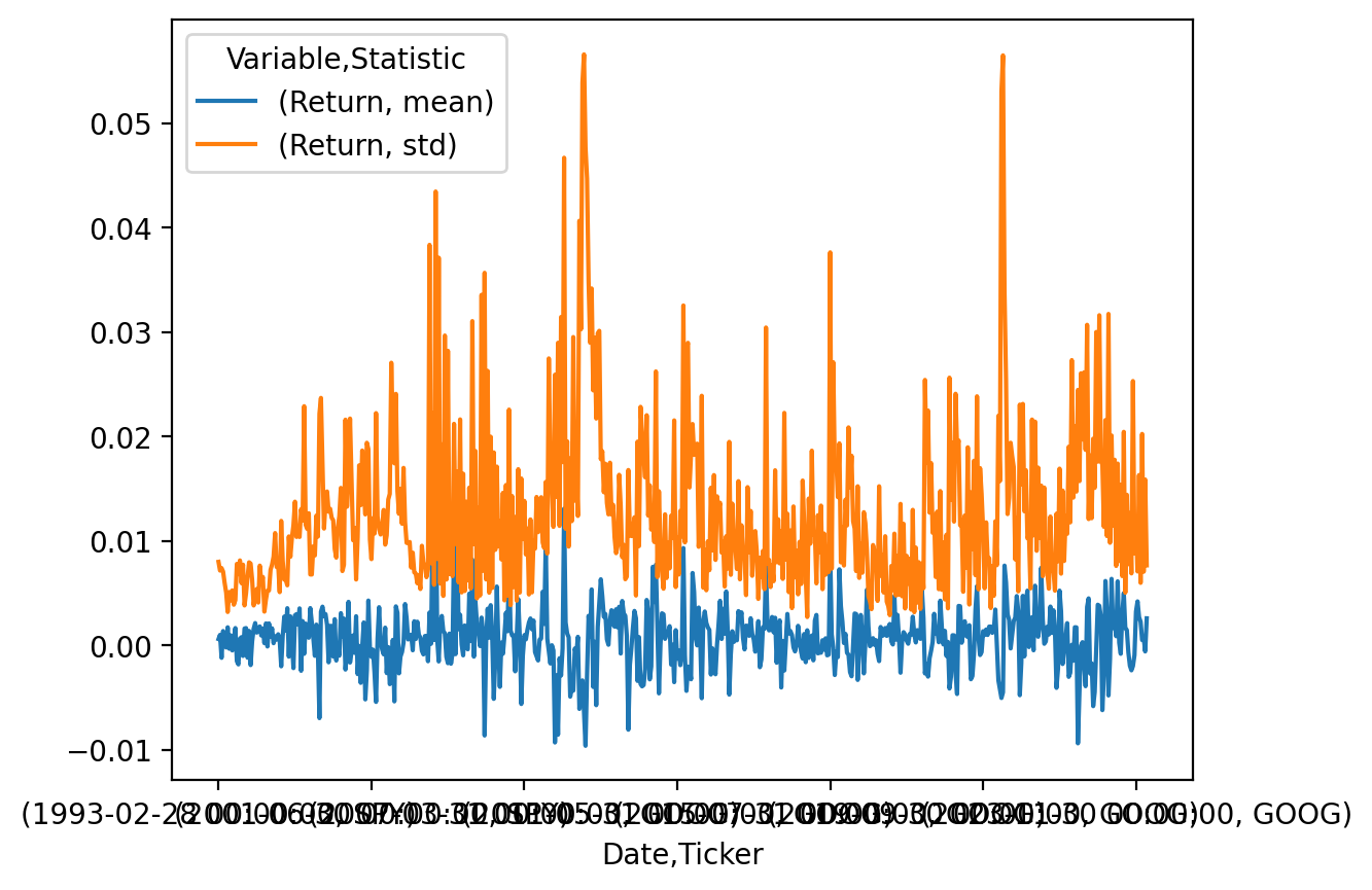
spy_goog_m.unstack().plot()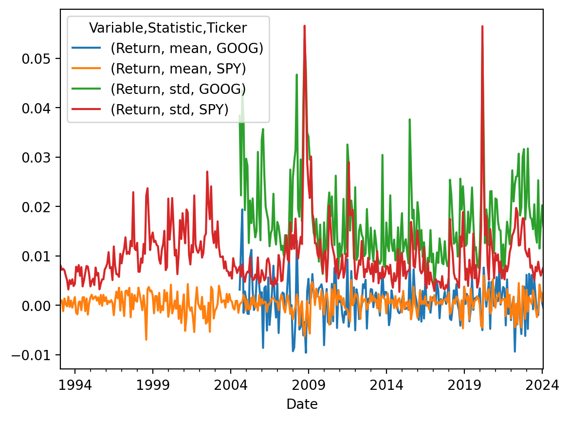
spy_goog_m.unstack().plot(subplots=True)array([<Axes: xlabel='Date'>, <Axes: xlabel='Date'>,
<Axes: xlabel='Date'>, <Axes: xlabel='Date'>], dtype=object)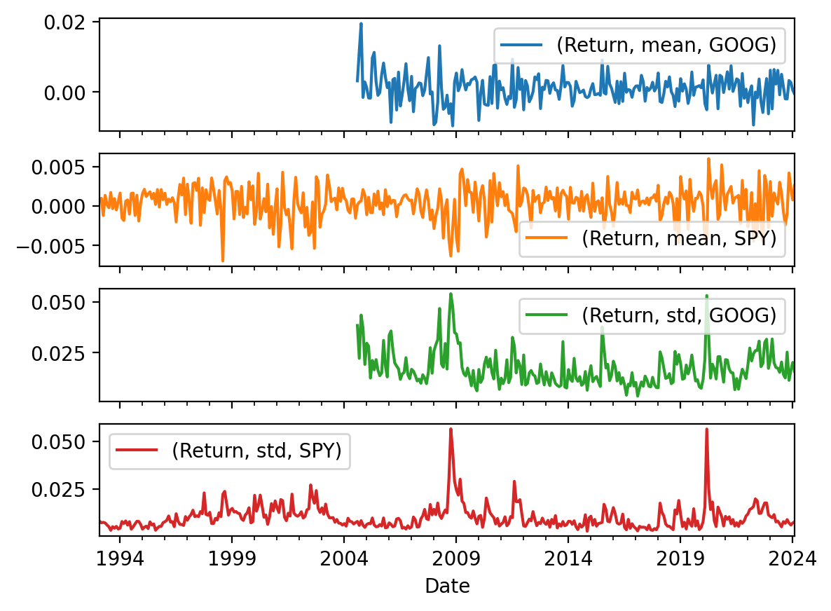
However, we have another excellent plotting tool in the seaborn package!
import seaborn as snsThe seaborn makes excellent multi-panel plots, including plots with statistics. But, it requires very long data frames. A very long data frame has all of the y values in one column and all other useful dimensions as columns instead of indexes!
sns.relplot(
    data=spy_goog_m.stack().reset_index(),
    x='Date',
    y='Return',
    kind='line',
    hue='Ticker',
    col='Statistic',
    height=3,
    alpha=0.75
)

plt.gcf().autofmt_xdate()
plt.suptitle('Monthly Mean and Volatility of Daily Returns', y=1.05)
plt.show()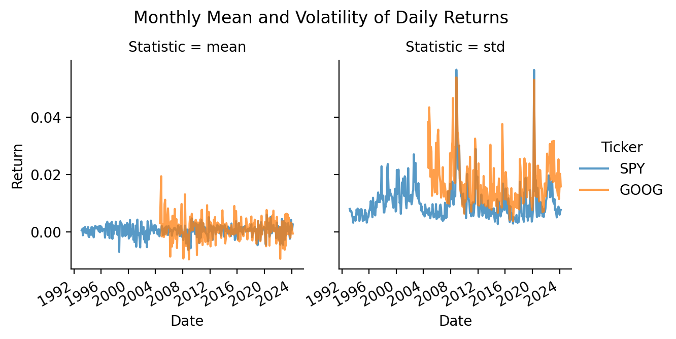
3.6 Assign the Dow Jones stocks to five portfolios based on their monthly volatility
wiki = pd.read_html('https://en.wikipedia.org/wiki/Dow_Jones_Industrial_Average')
wiki[1]['Symbol'].to_list()
['MMM',
'AXP',
'AMGN',
'AMZN',
'AAPL',
'BA',
'CAT',
'CVX',
'CSCO',
'KO',
'DIS',
'DOW',
'GS',
'HD',
'HON',
'IBM',
'INTC',
'JNJ',
'JPM',
'MCD',
'MRK',
'MSFT',
'NKE',
'PG',
'CRM',
'TRV',
'UNH',
'VZ',
'V',
'WMT']djia = (
yf.download(tickers=wiki[1]['Symbol'].to_list())
.rename_axis(columns=['Variable', 'Ticker'])
)
djia[*********************100%%**********************] 30 of 30 completed| Variable | Adj Close | ... | Volume | ||||||||||||||||||
|---|---|---|---|---|---|---|---|---|---|---|---|---|---|---|---|---|---|---|---|---|---|
| Ticker | AAPL | AMGN | AMZN | AXP | BA | CAT | CRM | CSCO | CVX | DIS | ... | MMM | MRK | MSFT | NKE | PG | TRV | UNH | V | VZ | WMT |
| Date | |||||||||||||||||||||
| 1962-01-02 | NaN | NaN | NaN | NaN | 0.1909 | 0.4767 | NaN | NaN | 0.3358 | 0.0582 | ... | 212800 | 633830 | NaN | NaN | 192000 | NaN | NaN | NaN | NaN | NaN |
| 1962-01-03 | NaN | NaN | NaN | NaN | 0.1947 | 0.4813 | NaN | NaN | 0.3350 | 0.0590 | ... | 422400 | 6564672 | NaN | NaN | 428800 | NaN | NaN | NaN | NaN | NaN |
| 1962-01-04 | NaN | NaN | NaN | NaN | 0.1928 | 0.4937 | NaN | NaN | 0.3320 | 0.0590 | ... | 212800 | 1199750 | NaN | NaN | 326400 | NaN | NaN | NaN | NaN | NaN |
| 1962-01-05 | NaN | NaN | NaN | NaN | 0.1890 | 0.4983 | NaN | NaN | 0.3236 | 0.0592 | ... | 315200 | 520646 | NaN | NaN | 544000 | NaN | NaN | NaN | NaN | NaN |
| 1962-01-08 | NaN | NaN | NaN | NaN | 0.1895 | 0.5014 | NaN | NaN | 0.3221 | 0.0590 | ... | 334400 | 1380845 | NaN | NaN | 1523200 | NaN | NaN | NaN | NaN | NaN |
| ... | ... | ... | ... | ... | ... | ... | ... | ... | ... | ... | ... | ... | ... | ... | ... | ... | ... | ... | ... | ... | ... |
| 2024-02-26 | 181.1600 | 286.3700 | 174.7300 | 216.9600 | 200.5400 | 325.3800 | 300.3900 | 48.4000 | 154.4500 | 107.6800 | ... | 3272900 | 5158400 | 16193500.0000 | 5831500.0000 | 4531900 | 1119800.0000 | 2308900.0000 | 3856900.0000 | 25108400.0000 | 32154800.0000 |
| 2024-02-27 | 182.6300 | 278.4900 | 173.5400 | 217.9800 | 201.4000 | 327.6300 | 299.5000 | 48.3100 | 152.1600 | 109.4200 | ... | 2288300 | 4780200 | 14835800.0000 | 5317400.0000 | 3868200 | 1245800.0000 | 3780600.0000 | 4145200.0000 | 17074100.0000 | 18012700.0000 |
| 2024-02-28 | 181.4200 | 277.4600 | 173.1600 | 218.0300 | 207.0000 | 329.5600 | 299.7700 | 48.0600 | 152.3400 | 110.8000 | ... | 2962400 | 5697200 | 13183100.0000 | 4219800.0000 | 3802900 | 965200.0000 | 9558600.0000 | 4358800.0000 | 12437000.0000 | 14803300.0000 |
| 2024-02-29 | 180.7500 | 273.8300 | 176.7600 | 219.4200 | 203.7200 | 333.9600 | 308.8200 | 48.3700 | 152.0100 | 111.5800 | ... | 5157700 | 11245800 | 31910700.0000 | 10810900.0000 | 8348100 | 1996600.0000 | 6832100.0000 | 6633700.0000 | 20485200.0000 | 29220100.0000 |
| 2024-03-01 | 179.6600 | 280.3300 | 178.2200 | 219.6600 | 200.0000 | 336.7000 | 316.8800 | 48.4000 | 152.8100 | 111.9500 | ... | 3390922 | 5990626 | 17596713.0000 | 7312382.0000 | 4814999 | 920132.0000 | 7107380.0000 | 3905662.0000 | 12084134.0000 | 18957132.0000 |
15648 rows × 180 columns
First, we add daily returns to djia.
_ = pd.MultiIndex.from_product([['Return'], djia['Adj Close']])
djia[_] = djia['Adj Close'].iloc[:-1].pct_change()
Second, we add monthly volatility of daily returns to each day. The .transform() methods lets us add monthly volatility to the original daily data.
_ = pd.MultiIndex.from_product([['Volatility'], djia['Return']])
djia[_] = djia['Return'].groupby(pd.Grouper(freq='M')).transform('std')
Third, we use pd.qcut() to assign stocks to portfolios based on volatility. Here is an example of how to use pd.qcut().
np.arange(10)array([0, 1, 2, 3, 4, 5, 6, 7, 8, 9])pd.qcut(
x=np.arange(10),
q=2,
labels=False
)array([0, 0, 0, 0, 0, 1, 1, 1, 1, 1], dtype=int64)We use the .apply() with axis=1 to apply pd.qcut to every row in djia['Volatility'] without writing a for loop. We can also pass q=5 and labels=False after we give the pd.qcut function name.
_ = pd.MultiIndex.from_product([['Portfolio'], djia['Volatility']])
djia[_] = djia['Volatility'].iloc[:-1].apply(pd.qcut, q=5, labels=False, axis=1)
3.7 Plot the time-series volatilities of these five portfolios
djia.stack()| Variable | Adj Close | Close | High | Low | Open | Volume | Return | Volatility | Portfolio | |
|---|---|---|---|---|---|---|---|---|---|---|
| Date | Ticker | |||||||||
| 1962-01-02 | BA | 0.1909 | 0.8230 | 0.8374 | 0.8230 | 0.8374 | 352350.0000 | NaN | 0.0156 | 3.0000 |
| CAT | 0.4767 | 1.6042 | 1.6198 | 1.5885 | 1.6042 | 163200.0000 | NaN | 0.0121 | 1.0000 | |
| CVX | 0.3358 | 3.2961 | 3.2961 | 3.2440 | 0.0000 | 105840.0000 | NaN | 0.0108 | 0.0000 | |
| DIS | 0.0582 | 0.0929 | 0.0960 | 0.0929 | 0.0929 | 841958.0000 | NaN | 0.0170 | 3.0000 | |
| HON | 1.0740 | 8.3100 | 8.3287 | 8.2726 | 0.0000 | 40740.0000 | NaN | 0.0097 | 0.0000 | |
| ... | ... | ... | ... | ... | ... | ... | ... | ... | ... | ... |
| 2024-03-01 | TRV | 218.8200 | 218.8200 | 221.0900 | 218.3900 | 220.7600 | 920132.0000 | NaN | NaN | NaN |
| UNH | 489.5300 | 489.5300 | 490.0200 | 477.2500 | 489.4200 | 7107380.0000 | NaN | NaN | NaN | |
| V | 283.1600 | 283.1600 | 284.9100 | 282.1100 | 283.2000 | 3905662.0000 | NaN | NaN | NaN | |
| VZ | 40.2000 | 40.2000 | 40.2900 | 39.7700 | 39.9900 | 12084134.0000 | NaN | NaN | NaN | |
| WMT | 58.7600 | 58.7600 | 58.8500 | 58.2000 | 58.8000 | 18957132.0000 | NaN | NaN | NaN |
351387 rows × 9 columns
(
    djia
    .stack()
    .groupby(['Date', 'Portfolio'])
    ['Return']
    .mean()
    .reset_index()
    .dropna()
    .assign(Portfolio=lambda x: x['Portfolio'].astype(int))
    .groupby([pd.Grouper(key='Date', freq='M'), 'Portfolio'])
    .std()
    .rename(columns={'Return': 'Volatility'})
    .unstack()
    ['Volatility']
    .plot()
)

plt.ylabel('Volatility of Daily Returns')
plt.title('Volatility of Daily Returns\n for Five Portfolios Formed Monthly on Volatility')
plt.show()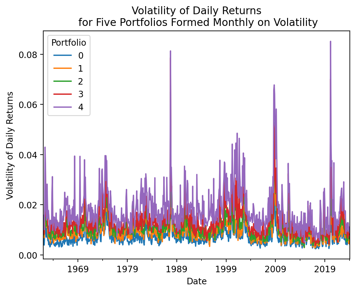
3.8 Calculate the mean monthly correlation between the Dow Jones stocks
I may build Project 2 on this exercise, so I will leave it blank, for now.
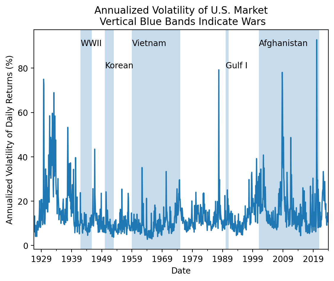
3.9 Is market volatility higher during wars?
Here is some guidance:
- Download the daily factor data from Ken French’s website
- Calculate daily market returns by summing the market risk premium and risk-free rates (
Mkt-RFandRF, respectively) - Calculate the volatility (standard deviation) of daily returns every month by combining
pd.Grouper()and.groupby()) - Multiply by \(\sqrt{252}\) to annualize these volatilities of daily returns
- Plot these annualized volatilities
Is market volatility higher during wars? Consider the following dates:
- WWII: December 1941 to September 1945
- Korean War: 1950 to 1953
- Viet Nam War: 1959 to 1975
- Gulf War: 1990 to 1991
- War in Afghanistan: 2001 to 2021
pdr.famafrench.get_available_datasets()[:5]['F-F_Research_Data_Factors',
'F-F_Research_Data_Factors_weekly',
'F-F_Research_Data_Factors_daily',
'F-F_Research_Data_5_Factors_2x3',
'F-F_Research_Data_5_Factors_2x3_daily']ff_all = pdr.DataReader(
name='F-F_Research_Data_Factors_daily',
data_source='famafrench',
start='1900'
)C:\Users\r.herron\AppData\Local\Temp\ipykernel_23660\2526882917.py:1: FutureWarning: The argument 'date_parser' is deprecated and will be removed in a future version. Please use 'date_format' instead, or read your data in as 'object' dtype and then call 'to_datetime'.
ff_all = pdr.DataReader((
ff_all[0]
.assign(Mkt = lambda x: x['Mkt-RF'] + x['RF'])
['Mkt']
.groupby(pd.Grouper(freq='M'))
.std()
.mul(np.sqrt(252))
.plot()
)
# adds vertical bands for U.S. wars
plt.axvspan('1941-12', '1945-09', alpha=0.25)
plt.annotate('WWII', ('1941-12', 90))
plt.axvspan('1950', '1953', alpha=0.25)
plt.annotate('Korean', ('1950', 80))
plt.axvspan('1959', '1975', alpha=0.25)
plt.annotate('Vietnam', ('1959', 90))
plt.axvspan('1990', '1991', alpha=0.25)
plt.annotate('Gulf I', ('1990', 80))
plt.axvspan('2001', '2021', alpha=0.25)
plt.annotate('Afghanistan', ('2001', 90))
plt.ylabel('Annualized Volatility of Daily Returns (%)')
plt.title('Annualized Volatility of U.S. Market\n Vertical Blue Bands Indicate Wars')
plt.show()