import matplotlib.pyplot as plt
import numpy as np
import pandas as pd
import yfinance as yfMcKinney Chapter 5 - Practice for Section 02
FINA 6333 for Spring 2024
1 Announcements
- No DataCamp this week, but I suggest you keep working on it
- Keep forming groups, and I will post our first project early next week
2 10-Minute Recap
%precision 4
pd.options.display.float_format = '{:.4f}'.format
%config InlineBackend.figure_format = 'retina'
There are two pandas data structures:
- Data frames are like worksheets in an Excel workbook (2-D, mixed data type)
- Series are like a column in a worksheet (1-D, only one data type)
np.random.seed(42)
df = pd.DataFrame(
    data=np.random.randn(3, 5),
    index=list('ABC'),
    columns=list('abcde')
)

df| a | b | c | d | e | |
|---|---|---|---|---|---|
| A | 0.4967 | -0.1383 | 0.6477 | 1.5230 | -0.2342 |
| B | -0.2341 | 1.5792 | 0.7674 | -0.4695 | 0.5426 |
| C | -0.4634 | -0.4657 | 0.2420 | -1.9133 | -1.7249 |
We can slice data frames two ways!
- By integer locations with the
.iloc[]method - By row and column names with the
.loc[]method
How can we grab the first 2 rows and 3 columns?
df.iloc[:2, :3] # pandas .iloc[] uses j,k notation, like NumPy| a | b | c | |
|---|---|---|---|
| A | 0.4967 | -0.1383 | 0.6477 |
| B | -0.2341 | 1.5792 | 0.7674 |
When we slice by names or string, pandas includes both left and right edges!
df.loc['A':'B', 'a':'c']| a | b | c | |
|---|---|---|---|
| A | 0.4967 | -0.1383 | 0.6477 |
| B | -0.2341 | 1.5792 | 0.7674 |
How can we add a column?
df['f'] = 2_001

df| a | b | c | d | e | f | |
|---|---|---|---|---|---|---|
| A | 0.4967 | -0.1383 | 0.6477 | 1.5230 | -0.2342 | 2001 |
| B | -0.2341 | 1.5792 | 0.7674 | -0.4695 | 0.5426 | 2001 |
| C | -0.4634 | -0.4657 | 0.2420 | -1.9133 | -1.7249 | 2001 |
What if we want to insert a column between “b” and “c”? We can use the .insert() method! Note. I was surprised the .insert() operates “in place” without an option to override!
df.insert(
    loc=2,
    column='C',
    value=5
)
df.loc[:, 'a':'c']| a | b | C | c | |
|---|---|---|---|---|
| A | 0.4967 | -0.1383 | 5 | 0.6477 |
| B | -0.2341 | 1.5792 | 5 | 0.7674 |
| C | -0.4634 | -0.4657 | 5 | 0.2420 |
df[['a', 'b', 'C', 'c']]| a | b | C | c | |
|---|---|---|---|---|
| A | 0.4967 | -0.1383 | 5 | 0.6477 |
| B | -0.2341 | 1.5792 | 5 | 0.7674 |
| C | -0.4634 | -0.4657 | 5 | 0.2420 |
A series is the other data structure in pandas!
ser = pd.Series(data=np.arange(2.), index=['B', 'C'])

ser
B 0.0000
C 1.0000
dtype: float64df['g'] = ser
df| a | b | C | c | d | e | f | g | |
|---|---|---|---|---|---|---|---|---|
| A | 0.4967 | -0.1383 | 5 | 0.6477 | 1.5230 | -0.2342 | 2001 | NaN |
| B | -0.2341 | 1.5792 | 5 | 0.7674 | -0.4695 | 0.5426 | 2001 | 0.0000 |
| C | -0.4634 | -0.4657 | 5 | 0.2420 | -1.9133 | -1.7249 | 2001 | 1.0000 |
3 Practice
tickers = 'AAPL IBM MSFT GOOG'
prices = yf.download(tickers=tickers)
[*********************100%%**********************] 4 of 4 completedreturns = (
prices['Adj Close'] # slice adj close column
.iloc[:-1] # drop last row with intra day prices, which are sometimes missing
.pct_change() # calculate returns
.dropna() # drop leading rows with at least one missing value
)
returns| AAPL | GOOG | IBM | MSFT | |
|---|---|---|---|---|
| Date | ||||
| 2004-08-20 | 0.0029 | 0.0794 | 0.0042 | 0.0029 |
| 2004-08-23 | 0.0091 | 0.0101 | -0.0070 | 0.0044 |
| 2004-08-24 | 0.0280 | -0.0414 | 0.0007 | 0.0000 |
| 2004-08-25 | 0.0344 | 0.0108 | 0.0042 | 0.0114 |
| 2004-08-26 | 0.0487 | 0.0180 | -0.0045 | -0.0040 |
| ... | ... | ... | ... | ... |
| 2024-01-26 | -0.0090 | 0.0010 | -0.0158 | -0.0023 |
| 2024-01-29 | -0.0036 | 0.0068 | -0.0015 | 0.0143 |
| 2024-01-30 | -0.0192 | -0.0116 | 0.0039 | -0.0028 |
| 2024-01-31 | -0.0194 | -0.0735 | -0.0224 | -0.0269 |
| 2024-02-01 | 0.0133 | 0.0064 | 0.0176 | 0.0156 |
4896 rows × 4 columns
returns = (
    prices['Adj Close']
    .iloc[:-1]
    .pct_change()
    .dropna()
)
returns| AAPL | GOOG | IBM | MSFT | |
|---|---|---|---|---|
| Date | ||||
| 2004-08-20 | 0.0029 | 0.0794 | 0.0042 | 0.0029 |
| 2004-08-23 | 0.0091 | 0.0101 | -0.0070 | 0.0044 |
| 2004-08-24 | 0.0280 | -0.0414 | 0.0007 | 0.0000 |
| 2004-08-25 | 0.0344 | 0.0108 | 0.0042 | 0.0114 |
| 2004-08-26 | 0.0487 | 0.0180 | -0.0045 | -0.0040 |
| ... | ... | ... | ... | ... |
| 2024-01-26 | -0.0090 | 0.0010 | -0.0158 | -0.0023 |
| 2024-01-29 | -0.0036 | 0.0068 | -0.0015 | 0.0143 |
| 2024-01-30 | -0.0192 | -0.0116 | 0.0039 | -0.0028 |
| 2024-01-31 | -0.0194 | -0.0735 | -0.0224 | -0.0269 |
| 2024-02-01 | 0.0133 | 0.0064 | 0.0176 | 0.0156 |
4896 rows × 4 columns
3.1 What are the mean daily returns for these four stocks?
returns.mean()AAPL 0.0014
GOOG 0.0010
IBM 0.0004
MSFT 0.0008
dtype: float64We if want an equally-weighted portfolio return? We could take the mean of each row with .mean(axis=1). The mean is the same as the sum of 0.25 times each of the 4 columns.
returns.mean(axis=1)Date
2004-08-20 0.0224
2004-08-23 0.0041
2004-08-24 -0.0032
2004-08-25 0.0152
2004-08-26 0.0146
...
2024-01-26 -0.0065
2024-01-29 0.0040
2024-01-30 -0.0074
2024-01-31 -0.0356
2024-02-01 0.0132
Length: 4896, dtype: float643.2 What are the standard deviations of daily returns for these four stocks?
returns.std()AAPL 0.0206
GOOG 0.0194
IBM 0.0143
MSFT 0.0171
dtype: float643.3 What are the annualized means and standard deviations of daily returns for these four stocks?
We multiply by \(T\) to annualize means, where \(T\) is the number of observations per year.
returns.mean().mul(252)AAPL 0.3625
GOOG 0.2552
IBM 0.0980
MSFT 0.2002
dtype: float64We multiply by \(\sqrt{T}\) to annualize volatilities, where \(T\) is the number of observations per year.
returns.std().mul(np.sqrt(252))AAPL 0.3276
GOOG 0.3074
IBM 0.2272
MSFT 0.2722
dtype: float643.4 Plot annualized means versus standard deviations of daily returns for these four stocks
Use plt.scatter(), which expects arguments as x (standard deviations) then y (means).
vols = returns.std().mul(np.sqrt(252) * 100)
means = returns.mean().mul(252 * 100)

plt.scatter(
    x=vols,
    y=means,
    c=['red', 'blue', 'green', 'purple']
)

plt.xlabel('Annualized Volatility of Daily Returns (%)')
plt.ylabel('Annualized Mean of Daily Returns (%)')

# plt.xlim((0, vols.max() + 5))
# plt.ylim((0, means.max() + 5))

# add tickers to each point
for i in means.index: # loop over ticker index
    plt.text( # plots string s at coordinates x and y
        x=vols[i], # indexes volatility
        y=means[i], # indexes mean return
        s=i # ticker index
    )

plt.title('Returns versus Risk')
plt.show() # suppresses output of last function call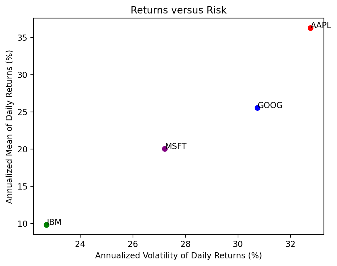
3.5 Repeat the previous calculations and plot for the stocks in the Dow-Jones Industrial Index (DJIA)
We can find the current DJIA stocks on Wikipedia. We will need to download new data, into tickers2, prices2, and returns2.
url2 = 'https://en.wikipedia.org/wiki/Dow_Jones_Industrial_Average'
wiki2 = pd.read_html(io=url2)
tickers2 = wiki2[1]['Symbol'].to_list()
tickers2[:5]
['MMM', 'AXP', 'AMGN', 'AAPL', 'BA']prices2 = yf.download(tickers=tickers2)[*********************100%%**********************] 30 of 30 completedreturns2 = (
prices2['Adj Close'] # slice the adj close columns for all 30 tickers
.iloc[:-1] # drop last row with incomplete prices because we are before the close
.pct_change() # calculate returns
.dropna() # drops any row with incomplete data
)
returns2| AAPL | AMGN | AXP | BA | CAT | CRM | CSCO | CVX | DIS | DOW | ... | MRK | MSFT | NKE | PG | TRV | UNH | V | VZ | WBA | WMT | |
|---|---|---|---|---|---|---|---|---|---|---|---|---|---|---|---|---|---|---|---|---|---|
| Date | |||||||||||||||||||||
| 2019-03-21 | 0.0368 | 0.0040 | 0.0095 | -0.0092 | 0.0079 | 0.0210 | 0.0128 | 0.0094 | -0.0121 | -0.0165 | ... | 0.0106 | 0.0230 | 0.0152 | 0.0076 | 0.0231 | 0.0061 | 0.0133 | 0.0108 | 0.0129 | 0.0043 |
| 2019-03-22 | -0.0207 | -0.0270 | -0.0211 | -0.0283 | -0.0320 | -0.0326 | -0.0222 | -0.0220 | -0.0040 | -0.0078 | ... | -0.0080 | -0.0264 | -0.0661 | -0.0081 | 0.0039 | -0.0196 | -0.0175 | 0.0252 | -0.0187 | -0.0079 |
| 2019-03-25 | -0.0121 | -0.0006 | -0.0038 | 0.0229 | 0.0124 | -0.0038 | -0.0002 | -0.0016 | -0.0041 | 0.0113 | ... | 0.0007 | 0.0052 | 0.0017 | 0.0030 | 0.0004 | -0.0009 | -0.0003 | 0.0054 | -0.0115 | -0.0011 |
| 2019-03-26 | -0.0103 | 0.0090 | 0.0042 | -0.0002 | 0.0035 | -0.0092 | 0.0095 | 0.0101 | 0.0218 | -0.0061 | ... | 0.0069 | 0.0021 | 0.0128 | 0.0104 | 0.0002 | -0.0141 | 0.0148 | 0.0092 | 0.0037 | 0.0015 |
| 2019-03-27 | 0.0090 | -0.0104 | -0.0047 | 0.0103 | -0.0049 | -0.0269 | -0.0017 | -0.0108 | 0.0013 | 0.0256 | ... | -0.0076 | -0.0097 | -0.0035 | -0.0012 | 0.0101 | -0.0069 | -0.0070 | 0.0041 | 0.0050 | -0.0113 |
| ... | ... | ... | ... | ... | ... | ... | ... | ... | ... | ... | ... | ... | ... | ... | ... | ... | ... | ... | ... | ... | ... |
| 2024-01-26 | -0.0090 | 0.0049 | 0.0710 | 0.0178 | -0.0045 | 0.0033 | -0.0036 | 0.0038 | 0.0053 | -0.0160 | ... | 0.0057 | -0.0023 | 0.0196 | 0.0033 | -0.0004 | 0.0199 | -0.0171 | 0.0026 | -0.0113 | 0.0088 |
| 2024-01-29 | -0.0036 | 0.0054 | -0.0028 | -0.0014 | 0.0128 | 0.0283 | 0.0029 | -0.0004 | 0.0223 | 0.0002 | ... | 0.0038 | 0.0143 | 0.0110 | 0.0001 | -0.0015 | 0.0027 | 0.0213 | -0.0083 | -0.0057 | 0.0047 |
| 2024-01-30 | -0.0192 | 0.0037 | 0.0164 | -0.0231 | 0.0050 | -0.0005 | -0.0010 | 0.0070 | -0.0056 | 0.0074 | ... | 0.0031 | -0.0028 | 0.0029 | 0.0085 | 0.0115 | -0.0018 | 0.0128 | 0.0100 | 0.0018 | 0.0033 |
| 2024-01-31 | -0.0194 | -0.0011 | -0.0167 | 0.0529 | -0.0146 | -0.0231 | -0.0394 | -0.0179 | -0.0092 | -0.0160 | ... | -0.0072 | -0.0269 | -0.0254 | -0.0022 | -0.0102 | 0.0161 | -0.0140 | -0.0028 | -0.0083 | -0.0021 |
| 2024-02-01 | 0.0133 | 0.0328 | 0.0124 | -0.0058 | 0.0246 | 0.0096 | 0.0000 | 0.0031 | 0.0105 | -0.0011 | ... | 0.0464 | 0.0156 | 0.0023 | 0.0130 | 0.0031 | -0.0090 | 0.0139 | 0.0033 | 0.0301 | 0.0185 |
1226 rows × 30 columns
vols2 = returns2.std().mul(np.sqrt(252) * 100)
means2 = returns2.mean().mul(252 * 100)

plt.scatter(
    x=vols2,
    y=means2
)

plt.xlabel('Annualized Volatility of Daily Returns (%)')
plt.ylabel('Annualized Mean of Daily Returns (%)')

# plt.xlim((0, vols2.max() + 5))
# plt.ylim((0, means2.max() + 5))

# add tickers to each point
for i in means2.index: # loop over ticker index
    plt.text( # plots string s at coordinates x and y
        x=vols2[i], # indexes volatility
        y=means2[i], # indexes mean return
        s=i # ticker index
    )

plt.title('Returns versus Risk')
plt.show() # suppresses output of last function call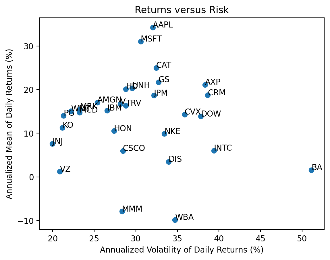
With 30 stocks we see there is no relation between returns and volatility because most volatility is diversifiable and uncompensated.
3.6 Calculate total returns for the stocks in the DJIA
We can use the .prod() method to compound returns as \(1 + R_T = \prod_{t=1}^T (1 + R_t)\). Technically, we should write \(R_T\) as \(R_{0,T}\), but we typically omit the subscript \(0\).
I prefer to chain these operations, with .add(1), then .prod(), then .sub(1).
total_returns2 = returns2.add(1).prod().sub(1)

total_returns2.iloc[:5]
AAPL 3.1210
AMGN 0.9635
AXP 0.9687
BA -0.4289
CAT 1.6083
dtype: float643.7 Plot the distribution of total returns for the stocks in the DJIA
We can plot a histogram, using either the plt.hist() function or the .plot(kind='hist') method.
A histogram is a great way to visualize data!
(
    returns2
    .add(1)
    .prod()
    .sub(1)
    .mul(100)
    .plot(kind='hist', bins=20)
)

start_date = returns2.index.min()
stop_date = returns2.index.max()

plt.xlabel('Total Return (%)')
plt.title(f'Distribution of Total Returns for DJIA Stocks\n from {start_date:%B %Y} through {stop_date:%B %Y}')
plt.show()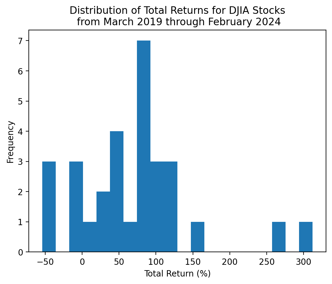
With only 30 stocks, we can actually visualize each total return!
(
    returns2
    .add(1)
    .prod()
    .sub(1)
    .sort_values() # sort by total returns
    .mul(100)
    .plot(kind='barh') # horizontal bar chart
)

start_date = returns2.index.min()
stop_date = returns2.index.max()

plt.xlabel('Total Return (%)')
plt.ylabel('Ticker')
plt.title(f'Distribution of Total Returns for DJIA Stocks\n from {start_date:%B %Y} through {stop_date:%B %Y}')
plt.show()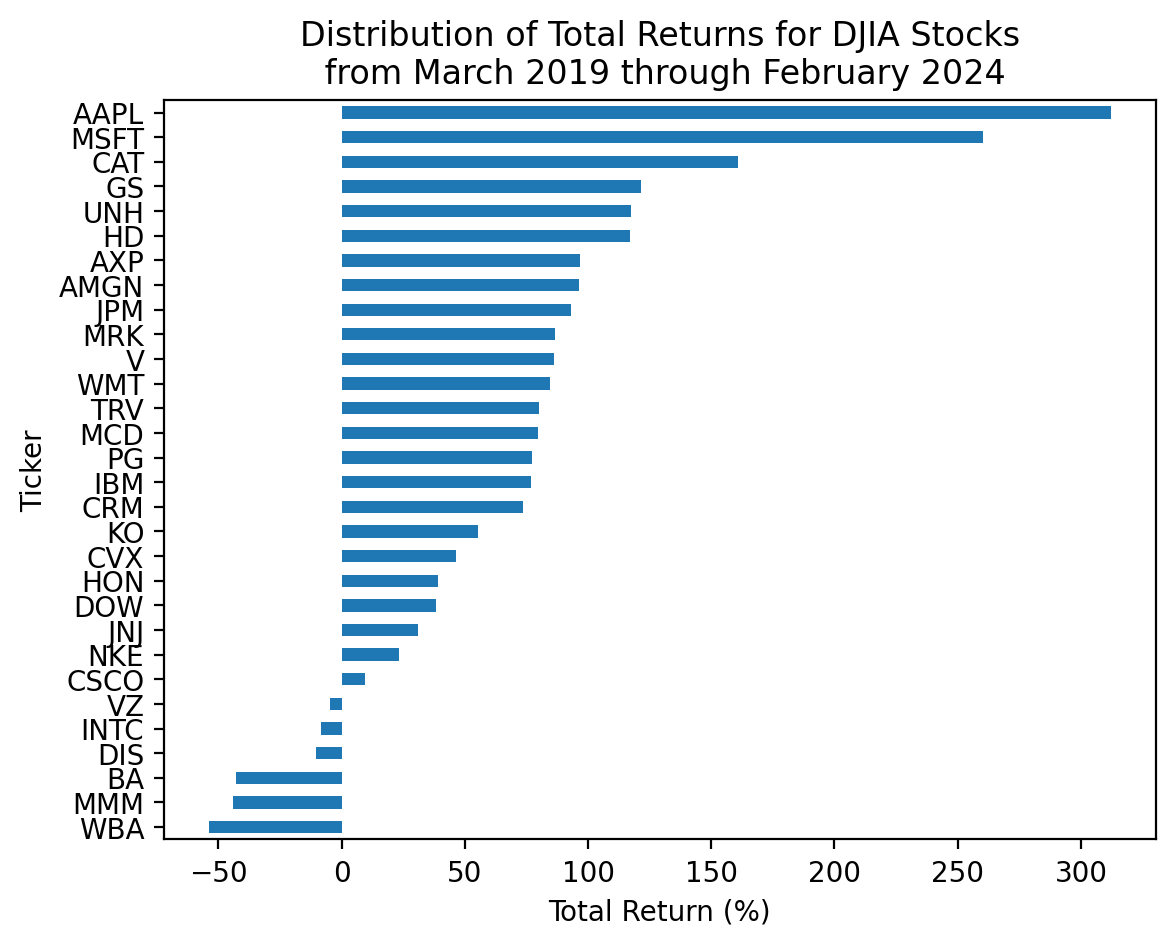
3.8 Which stocks have the minimum and maximum total returns?
If we want the values, the .min() and .max() methods are the way to go!
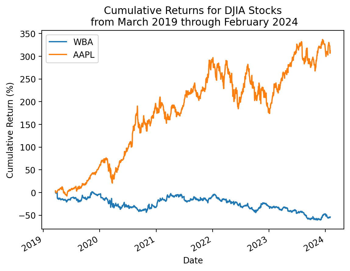
total_returns2.min()-0.5384total_returns2.max()3.1210If we want the ticker, the .idxmin() and .idxmax() methods are the way to go!
total_returns2.idxmin()'WBA'total_returns2.idxmax()'AAPL'If we want the smallest and the largest together, we can chain a few methods!
total_returns2.sort_values().iloc[[0, -1]]WBA -0.5384
AAPL 3.1210
dtype: float64Not the exactly right tool here, but the .nsmallest()' and.nlargest()` methods are really useful!
total_returns2.nsmallest(3)WBA -0.5384
MMM -0.4408
BA -0.4289
dtype: float64total_returns2.nlargest(3)AAPL 3.1210
MSFT 2.6028
CAT 1.6083
dtype: float643.9 Plot the cumulative returns for the stocks in the DJIA
We can use the cumulative product method .cumprod() to calculate the right hand side of the formula above.
(
    returns2
    .add(1)
    .cumprod()
    .sub(1)
    .mul(100)
    .plot(legend=False, linewidth=0.5) # with 30 stocks, this legend is too big to be useful
)
start_date = returns2.index.min()
stop_date = returns2.index.max()

plt.ylabel('Cumulative Return (%)')
plt.title(f'Cumulative Returns for DJIA Stocks\n from {start_date:%B %Y} through {stop_date:%B %Y}')
plt.show()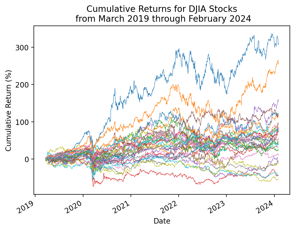
3.10 Repeat the plot above with only the minimum and maximum total returns
total_returns2.sort_values().iloc[[0, -1]].indexIndex(['WBA', 'AAPL'], dtype='object')(
returns2 # all returns for all stocks
[total_returns2.sort_values().iloc[[0, -1]].index] # slice min and max total return stocks
.add(1)
.cumprod()
.sub(1)
.mul(100)
.plot()
)
start_date = returns2.index.min()
stop_date = returns2.index.max()
plt.ylabel('Cumulative Return (%)')
plt.title(f'Cumulative Returns for DJIA Stocks\n from {start_date:%B %Y} through {stop_date:%B %Y}')
plt.show()