Herron Topic 5 - Practice for Section 04

FINA 6333 for Spring 2024

1 Practice

import matplotlib.pyplot as plt
import numpy as np
import pandas as pd
import pandas_datareader as pdr
import seaborn as sns
import yfinance as yf

%precision 2
pd.options.display.float_format = '{:.2f}'.format
%config InlineBackend.figure_format = 'retina'

1.1 Estimate \(\pi\) by simulating darts thrown at a dart board

Hints: Select random \(x\)s and \(y\)s such that \(-r \leq x \leq +r\) and \(-r \leq x \leq +r\). Darts are on the board if \(x^2 + y^2 \leq r^2\). The area of the circlular board is \(\pi r^2\), and the area of square around the board is \((2r)^2 = 4r^2\). The fraction \(f\) of darts on the board is the same as the ratio of circle area to square area, so \(f = \frac{\pi r^2}{4 r^2}\).

First we throw darts at the board. Darts with \(x^2 + y^2 \leq r^2\) are on the board.

def throw_darts(n=10_000, r=1, seed=42):
    np.random.seed(seed)
    return (
        pd.DataFrame(
            data=np.random.uniform(low=-r, high=r, size=2*n).reshape(n, 2), 
            columns=['x', 'y']
        )
        .assign(board=lambda x: x['x']**2 + x['y']**2 <= r**2)
        .rename_axis(index='n', columns='Variable')
    )

throw_darts()

Variable	x	y	board
n
0	-0.25	0.90	True
1	0.46	0.20	True
2	-0.69	-0.69	True
3	-0.88	0.73	False
4	0.20	0.42	True
...	...	...	...
9995	0.15	0.52	True
9996	-0.82	-0.01	True
9997	0.80	0.75	False
9998	-0.91	-0.39	True
9999	-0.11	-0.66	True

10000 rows × 3 columns

Next, we visualize these darts with a scatter plot. Seaborn’s scatterplot() helps color darts by location (i.e., on or off board). The .pipe() method lets us send the output of the .assign() method to sns.scatterplot() without assigning a temporary data frame.

(
    throw_darts()
    .assign(Location=lambda x: np.where(x['board'], 'On Board', 'Off Board'))
    .pipe(lambda x: sns.scatterplot(data=x, x='x', y='y', hue='Location'))
)
plt.title('Simulated Dart Throws')
plt.show()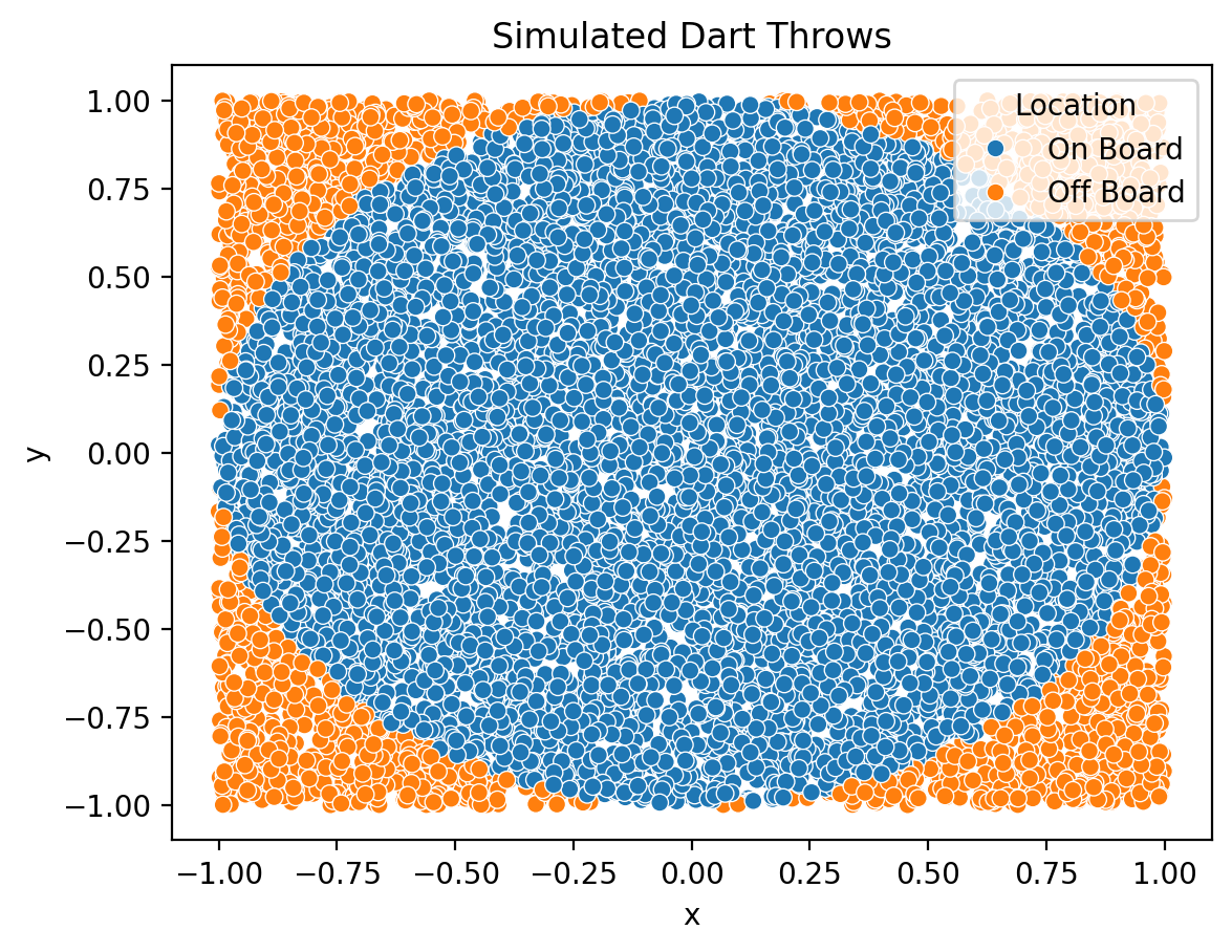

Finally, we use the hint above to estimate \(\pi\). The hint above says \(f = \frac{\pi r^2}{4 r^2}\), where \(f\) is the fraction of darts on the board. Therefore, \(\pi = \frac{4fr^2}{r^2} = 4f\).

n = 10_000
pi = 4 * throw_darts(n=n)["board"].mean()
print(f'Estimate of pi based on {n:,.0f} darts: {pi:0.4f}')

Estimate of pi based on 10,000 darts: 3.1544

We increase the precision of our \(\pi\) estimate by increasing the number of simulated darts \(n\).

for n in 10**np.arange(7):
    pi = 4 * throw_darts(n=n)["board"].mean()
    print(f'Estimate of pi based on {n:<9,.0f} darts: {pi:0.4f}')

Estimate of pi based on 1         darts: 4.0000
Estimate of pi based on 10        darts: 3.2000
Estimate of pi based on 100       darts: 3.0400
Estimate of pi based on 1,000     darts: 3.1040
Estimate of pi based on 10,000    darts: 3.1544
Estimate of pi based on 100,000   darts: 3.1468
Estimate of pi based on 1,000,000 darts: 3.1420

1.2 Simulate your wealth \(W_T\) by randomly sampling market returns

Use monthly market returns from the French Data Library. Only invest one cash flow \(W_0\), and plot the distribution of \(W_T\).

First, we download data from the French Data Library. We convert these returns from percent to decimal to simplify compounding.

mkt = (
    pdr.DataReader(
        name='F-F_Research_Data_Factors_daily',
        data_source='famafrench',
        start='1900'
    )[0]
    .assign(mkt=lambda x: (x['Mkt-RF'] + x['RF']) / 100)
    ['mkt']
)

C:\Users\r.herron\AppData\Local\Temp\ipykernel_13960\526361920.py:2: FutureWarning: The argument 'date_parser' is deprecated and will be removed in a future version. Please use 'date_format' instead, or read your data in as 'object' dtype and then call 'to_datetime'.
  pdr.DataReader(

Next, we write a couple of helper functions. The get_sample() function draws one random sample of n observations from returns series x. This sample provides one simulated return history.

pd.date_range

<function pandas.core.indexes.datetimes.date_range(start=None, end=None, periods=None, freq=None, tz=None, normalize: 'bool' = False, name: 'Hashable | None' = None, inclusive: 'IntervalClosedType' = 'both', *, unit: 'str | None' = None, **kwargs) -> 'DatetimeIndex'>

def get_sample(x, n=10_000, seed=42, start=None):
    if start is None:
        start = x.index[-1] + pd.offsets.BDay()
    return (
        x
        .sample(n=n, replace=True, random_state=seed, ignore_index=True)
        .set_axis(pd.date_range(start=start, periods=n, freq='B'))
        .rename_axis(index='Date')
    )    

The get_samples() function calls the get_sample() function m times to simulate m return histories. The get_samples() function combines these m return histories into one data frame.

def get_samples(x, m=100, n=10_000, seed=42, start=None):
    return (
        pd.concat(
            objs=[get_sample(x=x, n=n, seed=seed+i, start=start) for i in range(m)],
            axis=1,
            keys=range(m),
            names='Sample'
        )
    )

Next, we use these helper functions to simulate 100 return histories of 10,000 trading days each.

mkts = get_samples(x=mkt, m=100, n=10_000)
mkts

Sample	0	1	2	3	4	5	6	7	8	9	...	90	91	92	93	94	95	96	97	98	99
Date
2024-03-01	0.00	0.01	0.00	0.00	0.00	0.00	-0.00	0.00	-0.01	0.00	...	0.01	0.01	0.00	0.01	0.00	0.00	-0.00	-0.01	-0.01	0.00
2024-03-04	0.01	-0.00	0.00	0.01	0.00	-0.01	-0.01	0.01	0.00	-0.01	...	-0.00	0.00	0.01	-0.02	0.00	0.01	0.01	0.01	-0.01	-0.01
2024-03-05	-0.03	-0.00	-0.01	-0.03	-0.00	0.02	-0.00	0.00	-0.01	-0.01	...	0.00	-0.00	0.01	-0.02	-0.01	0.01	-0.00	0.00	-0.00	0.01
2024-03-06	-0.00	-0.00	-0.01	-0.00	0.01	0.01	0.00	-0.02	0.00	-0.01	...	0.01	-0.01	0.00	0.00	0.00	-0.02	-0.02	0.00	-0.00	0.01
2024-03-07	-0.00	-0.00	-0.00	-0.00	-0.01	-0.00	0.01	0.01	-0.00	0.01	...	0.00	-0.00	0.01	-0.01	-0.01	-0.03	-0.00	-0.01	-0.03	-0.00
...	...	...	...	...	...	...	...	...	...	...	...	...	...	...	...	...	...	...	...	...	...
2062-06-23	-0.01	0.00	0.00	0.00	0.00	0.03	-0.01	0.00	-0.00	0.01	...	-0.01	-0.01	0.00	0.00	-0.00	-0.07	0.01	0.02	-0.00	-0.00
2062-06-26	-0.00	0.01	-0.00	0.01	0.00	-0.01	0.01	0.00	-0.00	-0.00	...	0.00	-0.00	-0.01	-0.00	-0.01	0.00	0.01	0.01	0.03	-0.01
2062-06-27	-0.01	-0.01	0.02	-0.04	0.00	0.01	0.00	0.00	0.00	0.01	...	0.00	-0.00	-0.01	0.01	0.00	0.01	0.01	0.01	0.00	0.01
2062-06-28	-0.01	-0.01	0.00	-0.00	-0.01	-0.00	0.04	0.00	-0.00	-0.00	...	0.02	-0.00	-0.01	-0.01	-0.00	0.01	0.00	0.01	-0.00	-0.01
2062-06-29	-0.00	0.00	-0.01	0.01	-0.01	0.00	-0.01	-0.01	-0.01	0.00	...	-0.00	0.01	0.01	0.01	-0.00	0.00	-0.01	-0.02	0.01	-0.01

10000 rows × 100 columns

We compound daily returns \(R_t\) to find future wealth \(W_T\), so \(W_T = W_0 \times (1 + R_1) \times (1 + R_2) \times \cdots \times (1 + R_T)\). We use the .cumprod() method to compound the daily returns in data frame mkts.

W_0 = 1_000_000
W_t = W_0 * mkts.add(1).cumprod()

We visualize terminal wealth \(W_T\) with a cumulative distribution plot.

W_t.iloc[-1].plot(kind='hist', density=True, cumulative=True, bins=100)
plt.semilogx()
plt.xlabel(r'$W_T$ where $W_0 = $' + f'\\${W_0:,.0f}')
plt.title(r'Cumulative Distribution of $W_T$' + f'\nafter {W_t.shape[0]:,.0f} Trading Days')
plt.show()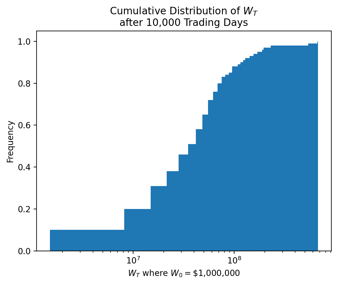

The plot above shows the cumulative distribution of \(W_T\), suggesting we expect \(W_T\) greater than about 20 million dollars for about 75% of samples. The plot above may be difficult to read and interpret because \(W_T\) has large outliers. The .describe() method provides few salient values of \(W_T\). We convert \(W_T\) from dollars to millions of dollars with .div(1_000_000).

W_t.iloc[-1].div(1_000_000).describe()

count   100.00
mean     61.07
std      90.71
min       1.50
25%      18.12
50%      41.47
75%      66.93
max     669.23
Name: 2062-06-29 00:00:00, dtype: float64

1.3 Repeat the exercise above but add end-of-month investments \(C_t\)

We can use the same data frame mkts of simulated market returns. However, need to consider end-of-month investments of \(C_t\). The easiest approach is to aggregate the daily market returns in mkts to monthly market returns in data frame mkts_m.

mkts_m = (
    mkts
    .add(1)
    .resample(rule='M', kind='period')
    .prod()
    .sub(1)
)

The wealth at time \(t\) is \(W_t\) and depends on:

1. The wealth at the end of the previous month \(W_{t-1}\)
2. The return over the previous month \(R_t\) (recall we label returns by their right edge)
3. The end-of-month investment \(C_t\)

Putting it all togther: \(W_t = W_{t-1} \times (1 + R_t) + C_t\)

We have to loop over the monthly returns in mkts_m because we have to combine compounded returns and cash flows. The iterrows() methods provides an easy way to iterate (loop) over the rows in mkts_m.

C_t = 1_000
W_0 = 1_000_000
W_last = W_0
W_t = []

for d, m in mkts_m.iterrows():
    W_last = (1 + m) * W_last + C_t
    W_t.append(W_last)

W_t = pd.concat(objs=W_t, axis=1, keys=mkts_m.index).transpose()

We repeat the cumulative distribution of wealth plot and descriptive statistics from above.

W_t.iloc[-1].plot(kind='hist', density=True, cumulative=True, bins=100)
plt.semilogx()
plt.xlabel(
    r'$W_T$ where $W_0 = $' + f'\\${W_0:,.0f}' + 
    r' and  $C_t = $' + f'\\${C_t:,.0f}'
)
plt.title(r'Cumulative Distribution of $W_T$' + f'\nafter {W_t.shape[0]:,.0f} Trading Months')
plt.show()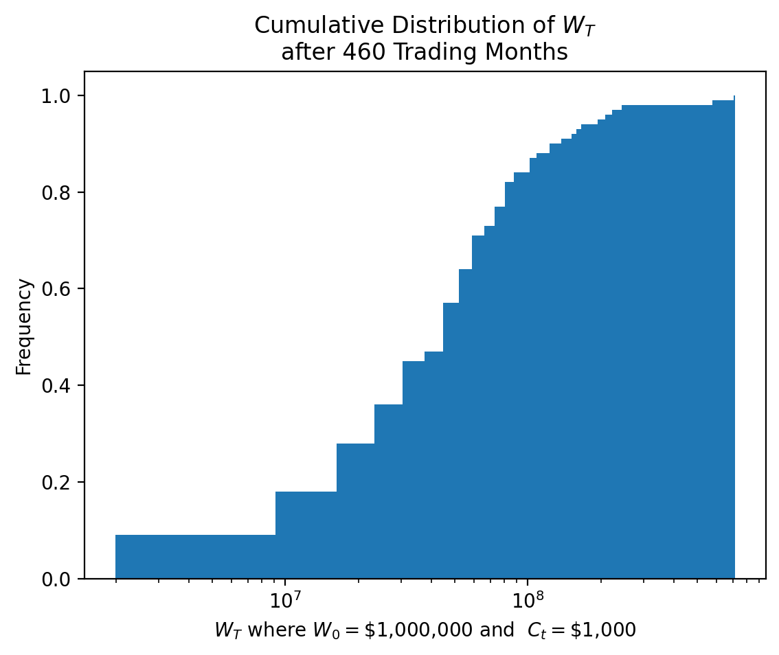

W_t.iloc[-1].div(1_000_000).describe()

count   100.00
mean     67.84
std      97.55
min       1.99
25%      21.21
50%      46.54
75%      75.92
max     713.85
Name: 2062-06, dtype: float64

The plot above shows the cumulative distribution of \(W_T\), suggesting we expect \(W_T\) greater than about 20 million dollars for about 75% of samples. Note, even though we deposit $1,000 per month for almost 40 years, we do not gain much wealth over the previous example with only a lump sum! Start saving early!