import matplotlib.pyplot as plt
import numpy as np
import pandas as pd
import pandas_datareader as pdr
import yfinance as yfHerron Topic 1 - Practice for Section 02
FINA 6333 for Spring 2024
1 Announcements
- DataCamp
- Data Manipulation with pandas due by Friday, 2/9, at 11:59 PM
- Joining Data with pandas due by Friday, 2/16, at 11:59 PM
- Earn 10,000 XP due by Friday, 3/15, at 11:59 PM
- I posted Project 1 to Canvas
- Slides and notebook due by Friday, 2/23, at 11:59 PM
- Keep joining teams and let me know if you need help
2 10-Minute Recap
%precision 4
pd.options.display.float_format = '{:.4f}'.format
%config InlineBackend.figure_format = 'retina'
First, we will use two packages to download data from the web:
yfinancefor Yahoo! Finance datapandas-datareaderfor Ken French data (and FRED data)
Second, there are “simple returns” and “log returns”
- Simple returns are the returns that investors receive that we learned in FINA 6331 and FINA 6333: \(r_t = \frac{p_t + d_t - p_{t-1}}{p_{t-1}}\)
- Log returns are the log of one plus simple returns. Why do we use them?
- Log returns are additive, while simple returns are multiplicative. This additive property makes math really easy with log returns: \(\log(\prod_{t=0}^T (1 + r_t)) = \sum_{t=0}^T \log(1+r_t)\), so \(r_{0,T} = \prod_{t=0}^T (1 + r_t) - 1 = e^{\sum_{t=0}^T \log(1+r_t)} - 1\)
- Log returns are almost normally distributed
We will almost always use simple returns. The exeception is time-consuming calculations, which we will often do in log returns to save us time.
Third, we can calculate portfolio returns a few ways
- We can calculate equally-weighted returns with
returns.mean(axis=1), rebalanced at the same frequency as returns - We can calculate any-weighted with
returns.dot(weights), whereweightsis an array of portfolio weights that are not necessarily equally-weighted, still rebalanced at the same frequency as returns
3 Practice
3.1 Download all available daily price data for tickers TSLA, F, AAPL, AMZN, and META to data frame prices
tickers = 'TSLA F AAPL AMZN META'
# tickers = ['TSLA', 'F',  'AAPL', 'AMZN', 'META']
prices = yf.download(tickers=tickers)

prices
[*********************100%%**********************] 5 of 5 completed| Adj Close | Close | ... | Open | Volume | |||||||||||||||||
|---|---|---|---|---|---|---|---|---|---|---|---|---|---|---|---|---|---|---|---|---|---|
| AAPL | AMZN | F | META | TSLA | AAPL | AMZN | F | META | TSLA | ... | AAPL | AMZN | F | META | TSLA | AAPL | AMZN | F | META | TSLA | |
| Date | |||||||||||||||||||||
| 1972-06-01 | NaN | NaN | 0.2419 | NaN | NaN | NaN | NaN | 2.1532 | NaN | NaN | ... | NaN | NaN | 0.0000 | NaN | NaN | NaN | NaN | 1091238 | NaN | NaN |
| 1972-06-02 | NaN | NaN | 0.2414 | NaN | NaN | NaN | NaN | 2.1492 | NaN | NaN | ... | NaN | NaN | 2.1532 | NaN | NaN | NaN | NaN | 1174468 | NaN | NaN |
| 1972-06-05 | NaN | NaN | 0.2414 | NaN | NaN | NaN | NaN | 2.1492 | NaN | NaN | ... | NaN | NaN | 2.1492 | NaN | NaN | NaN | NaN | 5209582 | NaN | NaN |
| 1972-06-06 | NaN | NaN | 0.2387 | NaN | NaN | NaN | NaN | 2.1248 | NaN | NaN | ... | NaN | NaN | 2.1492 | NaN | NaN | NaN | NaN | 1424158 | NaN | NaN |
| 1972-06-07 | NaN | NaN | 0.2373 | NaN | NaN | NaN | NaN | 2.1127 | NaN | NaN | ... | NaN | NaN | 2.1248 | NaN | NaN | NaN | NaN | 675088 | NaN | NaN |
| ... | ... | ... | ... | ... | ... | ... | ... | ... | ... | ... | ... | ... | ... | ... | ... | ... | ... | ... | ... | ... | ... |
| 2024-02-05 | 187.6800 | 170.3100 | 11.5900 | 459.4100 | 181.0600 | 187.6800 | 170.3100 | 11.5900 | 459.4100 | 181.0600 | ... | 188.1500 | 170.2000 | 12.0100 | 469.8800 | 184.2600 | 69668800.0000 | 55081300.0000 | 81026800 | 40832400.0000 | 134294400.0000 |
| 2024-02-06 | 189.3000 | 169.1500 | 12.0700 | 454.7200 | 185.1000 | 189.3000 | 169.1500 | 12.0700 | 454.7200 | 185.1000 | ... | 186.8600 | 169.3900 | 11.6400 | 464.0000 | 177.2100 | 43490800.0000 | 42505500.0000 | 98636800 | 21655200.0000 | 122676000.0000 |
| 2024-02-07 | 189.4100 | 170.5300 | 12.8000 | 469.5900 | 187.5800 | 189.4100 | 170.5300 | 12.8000 | 469.5900 | 187.5800 | ... | 190.6400 | 169.4800 | 12.7300 | 458.0000 | 188.1800 | 53439000.0000 | 47174100.0000 | 137224000 | 23066000.0000 | 111535200.0000 |
| 2024-02-08 | 188.3200 | 169.8400 | 12.8300 | 470.0000 | 189.5600 | 188.3200 | 169.8400 | 12.8300 | 470.0000 | 189.5600 | ... | 189.3900 | 169.6500 | 12.8700 | 468.3200 | 189.0000 | 40962000.0000 | 42316500.0000 | 68653900 | 18815100.0000 | 83034000.0000 |
| 2024-02-09 | 188.8500 | 174.4500 | 12.6800 | 468.1100 | 193.5700 | 188.8500 | 174.4500 | 12.6800 | 468.1100 | 193.5700 | ... | 188.6500 | 170.9000 | 12.8100 | 472.9500 | 190.1800 | 43728065.0000 | 56886544.0000 | 46925766 | 18159624.0000 | 84009121.0000 |
13035 rows × 30 columns
3.2 Calculate all available daily returns and save to data frame returns
returns = (
    prices['Adj Close'] # slice adj close
    .iloc[:-1] # drop the last price because it might be intraday (i.e., not a close)
    .pct_change() # calculate simple returns
)

returns| AAPL | AMZN | F | META | TSLA | |
|---|---|---|---|---|---|
| Date | |||||
| 1972-06-01 | NaN | NaN | NaN | NaN | NaN |
| 1972-06-02 | NaN | NaN | -0.0019 | NaN | NaN |
| 1972-06-05 | NaN | NaN | 0.0000 | NaN | NaN |
| 1972-06-06 | NaN | NaN | -0.0113 | NaN | NaN |
| 1972-06-07 | NaN | NaN | -0.0057 | NaN | NaN |
| ... | ... | ... | ... | ... | ... |
| 2024-02-02 | -0.0054 | 0.0787 | 0.0033 | 0.2032 | -0.0050 |
| 2024-02-05 | 0.0098 | -0.0087 | -0.0453 | -0.0328 | -0.0365 |
| 2024-02-06 | 0.0086 | -0.0068 | 0.0414 | -0.0102 | 0.0223 |
| 2024-02-07 | 0.0006 | 0.0082 | 0.0605 | 0.0327 | 0.0134 |
| 2024-02-08 | -0.0058 | -0.0040 | 0.0023 | 0.0009 | 0.0106 |
13034 rows × 5 columns
3.3 Slices returns for the 2020s and assign to returns_2020s
returns_2020s = returns.loc['2020':] # always use an unambiguos date format, like YYYY-MM-DD

returns_2020s| AAPL | AMZN | F | META | TSLA | |
|---|---|---|---|---|---|
| Date | |||||
| 2020-01-02 | 0.0228 | 0.0272 | 0.0129 | 0.0221 | 0.0285 |
| 2020-01-03 | -0.0097 | -0.0121 | -0.0223 | -0.0053 | 0.0296 |
| 2020-01-06 | 0.0080 | 0.0149 | -0.0054 | 0.0188 | 0.0193 |
| 2020-01-07 | -0.0047 | 0.0021 | 0.0098 | 0.0022 | 0.0388 |
| 2020-01-08 | 0.0161 | -0.0078 | 0.0000 | 0.0101 | 0.0492 |
| ... | ... | ... | ... | ... | ... |
| 2024-02-02 | -0.0054 | 0.0787 | 0.0033 | 0.2032 | -0.0050 |
| 2024-02-05 | 0.0098 | -0.0087 | -0.0453 | -0.0328 | -0.0365 |
| 2024-02-06 | 0.0086 | -0.0068 | 0.0414 | -0.0102 | 0.0223 |
| 2024-02-07 | 0.0006 | 0.0082 | 0.0605 | 0.0327 | 0.0134 |
| 2024-02-08 | -0.0058 | -0.0040 | 0.0023 | 0.0009 | 0.0106 |
1033 rows × 5 columns
What if we want a more complicated slice? We can combine .loc[] and Boolean conditions!
returns.loc[
    (returns.index.year == 2020) &
    ((returns.index.month == 1) | (returns.index.month == 12))
]| AAPL | AMZN | F | META | TSLA | |
|---|---|---|---|---|---|
| Date | |||||
| 2020-01-02 | 0.0228 | 0.0272 | 0.0129 | 0.0221 | 0.0285 |
| 2020-01-03 | -0.0097 | -0.0121 | -0.0223 | -0.0053 | 0.0296 |
| 2020-01-06 | 0.0080 | 0.0149 | -0.0054 | 0.0188 | 0.0193 |
| 2020-01-07 | -0.0047 | 0.0021 | 0.0098 | 0.0022 | 0.0388 |
| 2020-01-08 | 0.0161 | -0.0078 | 0.0000 | 0.0101 | 0.0492 |
| 2020-01-09 | 0.0212 | 0.0048 | 0.0011 | 0.0143 | -0.0219 |
| 2020-01-10 | 0.0023 | -0.0094 | -0.0011 | -0.0011 | -0.0066 |
| 2020-01-13 | 0.0214 | 0.0043 | -0.0011 | 0.0177 | 0.0977 |
| 2020-01-14 | -0.0135 | -0.0116 | 0.0054 | -0.0128 | 0.0249 |
| 2020-01-15 | -0.0043 | -0.0040 | -0.0108 | 0.0095 | -0.0361 |
| 2020-01-16 | 0.0125 | 0.0085 | -0.0022 | 0.0028 | -0.0097 |
| 2020-01-17 | 0.0111 | -0.0070 | -0.0011 | 0.0017 | -0.0058 |
| 2020-01-21 | -0.0068 | 0.0146 | 0.0055 | -0.0032 | 0.0719 |
| 2020-01-22 | 0.0036 | -0.0024 | -0.0054 | -0.0005 | 0.0409 |
| 2020-01-23 | 0.0048 | -0.0015 | -0.0022 | -0.0070 | 0.0046 |
| 2020-01-24 | -0.0029 | -0.0122 | -0.0153 | -0.0083 | -0.0129 |
| 2020-01-27 | -0.0294 | -0.0179 | -0.0122 | -0.0141 | -0.0120 |
| 2020-01-28 | 0.0283 | 0.0136 | 0.0090 | 0.0136 | 0.0159 |
| 2020-01-29 | 0.0209 | 0.0026 | 0.0045 | 0.0250 | 0.0249 |
| 2020-01-30 | -0.0014 | 0.0068 | -0.0023 | -0.0614 | 0.1030 |
| 2020-01-31 | -0.0443 | 0.0738 | -0.0023 | -0.0364 | 0.0152 |
| 2020-12-01 | 0.0308 | 0.0164 | 0.0176 | 0.0346 | 0.0302 |
| 2020-12-02 | 0.0029 | -0.0051 | -0.0043 | 0.0034 | -0.0273 |
| 2020-12-03 | -0.0011 | -0.0052 | 0.0011 | -0.0197 | 0.0432 |
| 2020-12-04 | -0.0056 | -0.0076 | 0.0141 | -0.0076 | 0.0095 |
| 2020-12-07 | 0.0123 | -0.0014 | -0.0128 | 0.0210 | 0.0713 |
| 2020-12-08 | 0.0051 | 0.0061 | 0.0033 | -0.0076 | 0.0127 |
| 2020-12-09 | -0.0209 | -0.0230 | 0.0216 | -0.0193 | -0.0699 |
| 2020-12-10 | 0.0120 | -0.0009 | -0.0349 | -0.0029 | 0.0374 |
| 2020-12-11 | -0.0067 | 0.0048 | -0.0110 | -0.0129 | -0.0272 |
| 2020-12-14 | -0.0051 | 0.0130 | -0.0122 | 0.0023 | 0.0489 |
| 2020-12-15 | 0.0501 | 0.0026 | 0.0269 | 0.0050 | -0.0103 |
| 2020-12-16 | -0.0005 | 0.0240 | -0.0120 | 0.0004 | -0.0165 |
| 2020-12-17 | 0.0070 | -0.0015 | 0.0044 | -0.0043 | 0.0532 |
| 2020-12-18 | -0.0159 | -0.0106 | -0.0143 | 0.0070 | 0.0596 |
| 2020-12-21 | 0.0124 | 0.0014 | -0.0022 | -0.0131 | -0.0649 |
| 2020-12-22 | 0.0285 | 0.0001 | -0.0157 | -0.0209 | -0.0146 |
| 2020-12-23 | -0.0070 | -0.0066 | 0.0228 | 0.0038 | 0.0088 |
| 2020-12-24 | 0.0077 | -0.0039 | -0.0145 | -0.0026 | 0.0244 |
| 2020-12-28 | 0.0358 | 0.0351 | 0.0034 | 0.0359 | 0.0029 |
| 2020-12-29 | -0.0133 | 0.0116 | -0.0079 | -0.0008 | 0.0035 |
| 2020-12-30 | -0.0085 | -0.0109 | 0.0045 | -0.0177 | 0.0432 |
| 2020-12-31 | -0.0077 | -0.0088 | -0.0079 | 0.0047 | 0.0157 |
3.4 Download all available data for the Fama and French daily benchmark factors to dictionary ff_all
I often use the following code snippet to find the exact name for the the daily benchmark factors file.
pdr.famafrench.get_available_datasets()[:5]['F-F_Research_Data_Factors',
'F-F_Research_Data_Factors_weekly',
'F-F_Research_Data_Factors_daily',
'F-F_Research_Data_5_Factors_2x3',
'F-F_Research_Data_5_Factors_2x3_daily']ff_all = pdr.DataReader(
name='F-F_Research_Data_Factors_daily',
data_source='famafrench',
start='1900'
)C:\Users\r.herron\AppData\Local\Temp\ipykernel_28696\2526882917.py:1: FutureWarning: The argument 'date_parser' is deprecated and will be removed in a future version. Please use 'date_format' instead, or read your data in as 'object' dtype and then call 'to_datetime'.
ff_all = pdr.DataReader(The DESCR key in the dictionary tells us about the data frames that pandas-datareader returns.
print(ff_all['DESCR'])F-F Research Data Factors daily
-------------------------------
This file was created by CMPT_ME_BEME_RETS_DAILY using the 202312 CRSP database. The Tbill return is the simple daily rate that, over the number of trading days in the month, compounds to 1-month TBill rate from Ibbotson and Associates Inc. Copyright 2023 Kenneth R. French
0 : (25649 rows x 4 cols)3.5 Slice the daily benchmark factors, convert them to decimal returns, and assign to ff
ff = ff_all[0].div(100)

ff| Mkt-RF | SMB | HML | RF | |
|---|---|---|---|---|
| Date | ||||
| 1926-07-01 | 0.0010 | -0.0025 | -0.0027 | 0.0001 |
| 1926-07-02 | 0.0045 | -0.0033 | -0.0006 | 0.0001 |
| 1926-07-06 | 0.0017 | 0.0030 | -0.0039 | 0.0001 |
| 1926-07-07 | 0.0009 | -0.0058 | 0.0002 | 0.0001 |
| 1926-07-08 | 0.0021 | -0.0038 | 0.0019 | 0.0001 |
| ... | ... | ... | ... | ... |
| 2023-12-22 | 0.0021 | 0.0064 | 0.0009 | 0.0002 |
| 2023-12-26 | 0.0048 | 0.0069 | 0.0046 | 0.0002 |
| 2023-12-27 | 0.0016 | 0.0014 | 0.0012 | 0.0002 |
| 2023-12-28 | -0.0001 | -0.0036 | 0.0003 | 0.0002 |
| 2023-12-29 | -0.0043 | -0.0112 | -0.0037 | 0.0002 |
25649 rows × 4 columns
3.6 Use the .cumprod() method to plot cumulative returns for these stocks in the 2020s
We use the .prod() method to calculate total returns, because \(r_{total} = r_{0,T} = \left[ \prod_{t=0}^T (1 + r_t) \right] -1\).
totret = (
    returns_2020s # returns during the 2020s
    .add(1) # add 1 before we compound
    .prod() # compound all returns
    .sub(1) # subtract 1 to recover total returns
)

totret
AAPL 1.6331
AMZN 0.8383
F 0.6090
META 1.2899
TSLA 5.7970
dtype: float64cumret_cumprod = returns_2020s.add(1).cumprod().sub(1)The last row in the cumulative returns data frame cumret_cumprod is the same as the total returns series totret!
np.allclose(totret, cumret_cumprod.iloc[-1])TrueWe can use the .plot() method to plot these cumulative returns!
cumret_cumprod.mul(100).plot()

# https://stackoverflow.com/questions/25973581/how-to-format-axis-number-format-to-thousands-with-a-comma
from matplotlib import ticker
plt.gca().get_yaxis().set_major_formatter(ticker.FuncFormatter(lambda x, p: format(int(x), ',')))

plt.ylabel('Cumulative Return (%)')
plt.title(f'Cumulative Returns\n from {cumret_cumprod.index.min():%b %Y} to {cumret_cumprod.index.max():%b %Y}')
plt.show()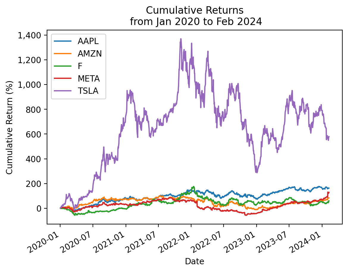
We can also plt.plot(), but lose a few of the formatting defaults built into the pandas method .plot().
plt.plot(cumret_cumprod.mul(100))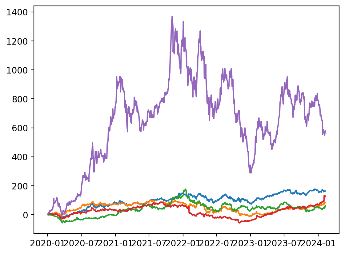
3.7 Use the .cumsum() method with log returns to plot cumulative returns for these stocks in the 2020s
cumret_cumsum = (
    returns_2020s
    .pipe(np.log1p) # converts simple returns to log returns
    .cumsum() # log returns are additive
    .pipe(np.expm1) # converts log returns to simple returns
)
# cumret_cumsum = returns_2020s.add(1).pipe(np.log).cumsum().pipe(np.exp).sub(1)
np.allclose(totret, cumret_cumsum.iloc[-1])Truecumret_cumsum.mul(100).plot()
# https://stackoverflow.com/questions/25973581/how-to-format-axis-number-format-to-thousands-with-a-comma
from matplotlib import ticker
plt.gca().get_yaxis().set_major_formatter(ticker.FuncFormatter(lambda x, p: format(int(x), ',')))
plt.ylabel('Cumulative Return (%)')
plt.title(f'Cumulative Returns\n from {cumret_cumsum.index.min():%b %Y} to {cumret_cumsum.index.max():%b %Y}')
plt.show()
3.8 Use price data only to plot cumulative returns for these stocks in the 2020s
We can also calculate cumulative returns as the ratio of adjusted closes. That is \(R_{0,T} = \frac{AC_T}{AC_0} - 1\). The trick here is that \(FV_t = PV (1+r)^t\), so \((1+r)^t = \frac{FV_t}{PV}\).
returns_2020s.iloc[0]AAPL 0.0228
AMZN 0.0272
F 0.0129
META 0.0221
TSLA 0.0285
Name: 2020-01-02 00:00:00, dtype: float64Note: We drop the last row in prices['Adj Close'] with .iloc[:-1]. We drop this last row here here because we did the same above when we calculated returns to exclude possible intraday returns.
cumret_prices = prices['Adj Close'].loc['2020':].iloc[:-1] / prices['Adj Close'].loc['2019'].iloc[-1] - 1

cumret_prices.iloc[0]
AAPL 0.0228
AMZN 0.0272
F 0.0129
META 0.0221
TSLA 0.0285
Name: 2020-01-02 00:00:00, dtype: float64np.allclose(cumret_cumprod, cumret_prices)Truecumret_prices.mul(100).plot()
# https://stackoverflow.com/questions/25973581/how-to-format-axis-number-format-to-thousands-with-a-comma
from matplotlib import ticker
plt.gca().get_yaxis().set_major_formatter(ticker.FuncFormatter(lambda x, p: format(int(x), ',')))
plt.ylabel('Cumulative Return (%)')
plt.title(f'Cumulative Returns\n from {cumret_prices.index.min():%b %Y} to {cumret_prices.index.max():%b %Y}')
plt.show()
3.9 Calculate the Sharpe Ratio for TSLA
Calculate the Sharpe Ratio with all available returns and 2020s returns. Recall the Sharpe Ratio is \(\frac{\overline{r_i - r_f}}{\sigma_i}\), where \(\sigma_i\) is the volatility of excess returns.
I suggest you write a function named calc_sharpe() to use for the rest of this notebook.
def calc_sharpe(ri, rf=ff['RF'], ppy=252):
    ri_rf = ri.sub(rf).dropna()
return np.sqrt(ppy) * ri_rf.mean() / ri_rf.std()calc_sharpe(ri=returns['TSLA'])0.9261calc_sharpe(ri=returns_2020s['TSLA'])1.1212We can use the .pipe() method here, too, since ri is the first argument to calc_sharpe()!
returns['TSLA'].pipe(calc_sharpe)0.9261returns_2020s['TSLA'].pipe(calc_sharpe)1.12123.10 Calculate the market beta for TSLA
Calculate the market beta with all available returns and 2020s returns. Recall we estimate market beta with the ordinary least squares (OLS) regression \(R_i-R_f = \alpha + \beta (R_m-R_f) + \epsilon\). We can estimate market beta with the covariance formula (i.e., \(\beta_i = \frac{Cov(R_i - R_f, R_m - R_f)}{Var(R_m-R_f)}\)) above for a univariate regression if we do not need goodness of fit statistics.
I suggest you write a function named calc_beta() to use for the rest of this notebook.
def calc_beta(ri, rf=ff['RF'], rm_rf=ff['Mkt-RF']):
    ri_rf = ri.sub(rf).dropna()
    rm_rf = rm_rf.loc[ri_rf.index]
return ri_rf.cov(rm_rf) / rm_rf.var()calc_beta(ri=returns['TSLA'])1.4417calc_beta(ri=returns_2020s['TSLA'])1.5780We can use the .pipe() method here, too, since ri is the first argument to calc_beta()!
returns['TSLA'].pipe(calc_beta)1.4417returns_2020s['TSLA'].pipe(calc_beta)1.57803.11 Guess the Sharpe Ratios for these stocks in the 2020s
3.12 Guess the market betas for these stocks in the 2020s
3.13 Calculate the Sharpe Ratios for these stocks in the 2020s
How good were your guesses?
for i in returns_2020s:
    sharpe_i = returns_2020s[i].pipe(calc_sharpe)
    print(f'Sharpe Ratio for {i}:\t {sharpe_i:0.2f}')
Sharpe Ratio for AAPL: 0.86
Sharpe Ratio for AMZN: 0.48
Sharpe Ratio for F: 0.42
Sharpe Ratio for META: 0.49
Sharpe Ratio for TSLA: 1.12We can also use pandas notation to vectorize this calculation. First calculate excess returns as \(r_i - r_f\).
returns_2020s_excess = returns_2020s.sub(ff['RF'], axis=0).dropna()Then use pandas notation to calculate means, standard deviations, and annualize.
(
    returns_2020s_excess
    .mean()
    .div(returns_2020s_excess.std())
    .mul(np.sqrt(252))
)
AAPL 0.8576
AMZN 0.4750
F 0.4240
META 0.4949
TSLA 1.1212
dtype: float64Note: In a few weeks we will learn the .apply() method, which avoids the loop syntax.
returns_2020s.apply(calc_sharpe)AAPL 0.8576
AMZN 0.4750
F 0.4240
META 0.4949
TSLA 1.1212
dtype: float643.14 Calculate the market betas for these stocks in the 2020s
How good were your guesses?
for i in returns_2020s:
    beta_i = returns_2020s[i].pipe(calc_beta)
    print(f'Beta for {i}:\t {beta_i:0.2f}')
Beta for AAPL: 1.15
Beta for AMZN: 1.04
Beta for F: 1.22
Beta for META: 1.27
Beta for TSLA: 1.58Or we can follow out approach above to vectorize this calculation. First, we need to add a market excess return column to returns_2020s_excess.
returns_2020s_excess['Mkt-RF'] = ff['Mkt-RF']
returns_2020s_excess.head()| AAPL | AMZN | F | META | TSLA | Mkt-RF | |
|---|---|---|---|---|---|---|
| Date | ||||||
| 2020-01-02 | 0.0228 | 0.0271 | 0.0128 | 0.0220 | 0.0285 | 0.0086 |
| 2020-01-03 | -0.0098 | -0.0122 | -0.0224 | -0.0054 | 0.0296 | -0.0067 |
| 2020-01-06 | 0.0079 | 0.0148 | -0.0055 | 0.0188 | 0.0192 | 0.0036 |
| 2020-01-07 | -0.0048 | 0.0020 | 0.0098 | 0.0021 | 0.0387 | -0.0019 |
| 2020-01-08 | 0.0160 | -0.0079 | -0.0001 | 0.0101 | 0.0491 | 0.0047 |
vcv = returns_2020s_excess.cov()
vcv| AAPL | AMZN | F | META | TSLA | Mkt-RF | |
|---|---|---|---|---|---|---|
| AAPL | 0.0004 | 0.0003 | 0.0002 | 0.0004 | 0.0005 | 0.0003 |
| AMZN | 0.0003 | 0.0006 | 0.0002 | 0.0004 | 0.0005 | 0.0002 |
| F | 0.0002 | 0.0002 | 0.0009 | 0.0003 | 0.0005 | 0.0003 |
| META | 0.0004 | 0.0004 | 0.0003 | 0.0009 | 0.0005 | 0.0003 |
| TSLA | 0.0005 | 0.0005 | 0.0005 | 0.0005 | 0.0018 | 0.0003 |
| Mkt-RF | 0.0003 | 0.0002 | 0.0003 | 0.0003 | 0.0003 | 0.0002 |
vcv['Mkt-RF'].div(vcv.loc['Mkt-RF', 'Mkt-RF']).plot(kind='bar')
plt.xlabel('Ticker')
plt.ylabel('CAPM Beta')
plt.title('CAPM Betas')
plt.show()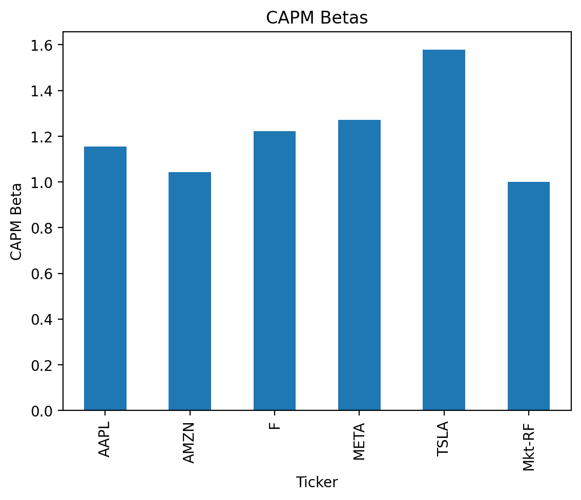
Note: In a few weeks we will learn the .apply() method, which avoids the loop syntax.
returns_2020s.apply(calc_beta)AAPL 1.1541
AMZN 1.0429
F 1.2231
META 1.2710
TSLA 1.5780
dtype: float643.15 Calculate the Sharpe Ratio for an equally weighted portfolio of these stocks in the 2020s
What do you notice?
returns_2020s.mean(axis=1).pipe(calc_sharpe)0.9573Because diversification reduces portfolio standard deviation less than the sum of its parts, the Sharpe Ratio of the equally weighted portfolio is less than the equally weighted mean of the single-stock Sharpe Ratios.
returns_2020s.apply(calc_sharpe).mean()0.67453.16 Calculate the market beta for an equally weighted portfolio of these stocks in the 2020s
What do you notice?
Beta measures nondiversifiable risk, so \(\beta_P = \sum w_i \beta_i\)!
returns_2020s.mean(axis=1).pipe(calc_beta)1.2538returns_2020s.apply(calc_beta).mean()1.25383.17 Calculate the market betas for these stocks every calendar year for every possible year
Save these market betas to data frame betas. Our current Python knowledge limits us to a for-loop, but we will learn easier and faster approaches soon!
betas = pd.DataFrame(
    index=range(1972, 2024),
    columns=returns.columns
)

betas.columns.name = 'Ticker'
betas.index.name = 'Year'

betas.tail()| Ticker | AAPL | AMZN | F | META | TSLA |
|---|---|---|---|---|---|
| Year | |||||
| 2019 | NaN | NaN | NaN | NaN | NaN |
| 2020 | NaN | NaN | NaN | NaN | NaN |
| 2021 | NaN | NaN | NaN | NaN | NaN |
| 2022 | NaN | NaN | NaN | NaN | NaN |
| 2023 | NaN | NaN | NaN | NaN | NaN |
for i in betas.index:
    for c in betas.columns:
        betas.at[i, c] = returns.loc[str(i), c].pipe(calc_beta)

betas.tail()| Ticker | AAPL | AMZN | F | META | TSLA |
|---|---|---|---|---|---|
| Year | |||||
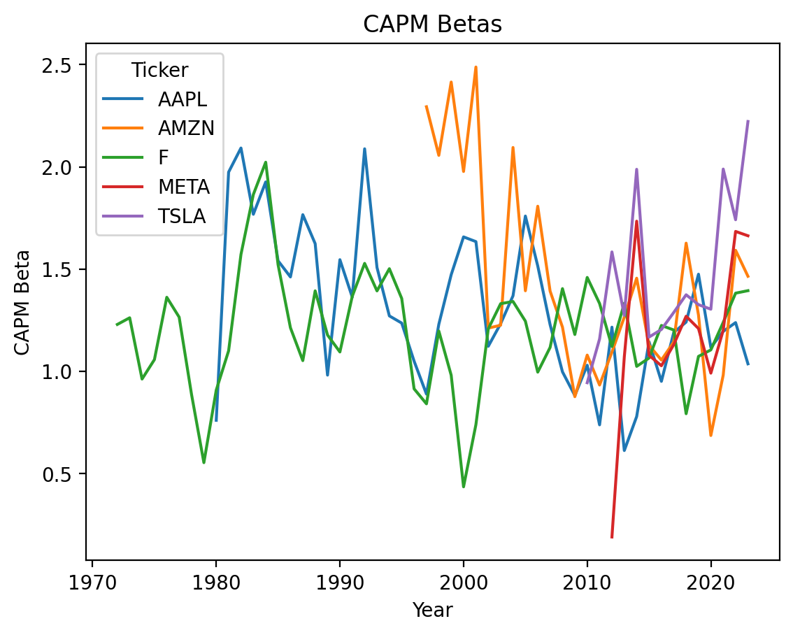
| 2019 | 1.4751 | 1.2752 | 1.0733 | 1.2094 | 1.3262 |
| 2020 | 1.1174 | 0.6866 | 1.1052 | 0.9913 | 1.3041 |
| 2021 | 1.1957 | 0.9822 | 1.2396 | 1.2014 | 1.9891 |
| 2022 | 1.2386 | 1.5922 | 1.3824 | 1.6843 | 1.7414 |
| 2023 | 1.0369 | 1.4649 | 1.3947 | 1.6630 | 2.2218 |
3.18 Plot the time series of market betas
betas.plot()
plt.ylabel('CAPM Beta')
plt.title('CAPM Betas')
plt.show()