import matplotlib.pyplot as plt
import matplotlib.ticker as ticker
import numpy as np
import pandas as pd
import pandas_datareader as pdr
import seaborn as sns
import statsmodels.api as sm
import yfinance as yfHerron Topic 2 - Practice for Section 02
FINA 6333 for Spring 2024
1 Announcements
- Project 2 is due Friday, 3/29, at 11:59 PM
- We will dedicate class next week to group work and easy access to me (i.e., no pre-class quiz)
2 10-Minute Recap
- Technical analysis studies market trends to estimate where prices may go. It looks for patterns in past price moves and trade volumes, and traders use these signals to inform their trades.
- There is little evidence that technical analysis works, but it provides a context for us to introduce quantitative investing strategies.
- We should never base trades on information we do not have at the time of the trade!
3 Practice
%precision 4
pd.options.display.float_format = '{:.4f}'.format
%config InlineBackend.figure_format = 'retina'
3.1 Implement the SMA(20) strategy with Bitcoin from the lecture notebook
I suggest writing a function calc_sma() that accepts a data frame df and moving average window n. First, we need the data, from ticker BTC-USD from Yahoo! Finance.
btc = (
    yf.download('BTC-USD')
    .rename_axis(columns='Variable')
)

btc.head(10)
[*********************100%%**********************] 1 of 1 completed| Variable | Open | High | Low | Close | Adj Close | Volume |
|---|---|---|---|---|---|---|
| Date | ||||||
| 2014-09-17 | 465.8640 | 468.1740 | 452.4220 | 457.3340 | 457.3340 | 21056800 |
| 2014-09-18 | 456.8600 | 456.8600 | 413.1040 | 424.4400 | 424.4400 | 34483200 |
| 2014-09-19 | 424.1030 | 427.8350 | 384.5320 | 394.7960 | 394.7960 | 37919700 |
| 2014-09-20 | 394.6730 | 423.2960 | 389.8830 | 408.9040 | 408.9040 | 36863600 |
| 2014-09-21 | 408.0850 | 412.4260 | 393.1810 | 398.8210 | 398.8210 | 26580100 |
| 2014-09-22 | 399.1000 | 406.9160 | 397.1300 | 402.1520 | 402.1520 | 24127600 |
| 2014-09-23 | 402.0920 | 441.5570 | 396.1970 | 435.7910 | 435.7910 | 45099500 |
| 2014-09-24 | 435.7510 | 436.1120 | 421.1320 | 423.2050 | 423.2050 | 30627700 |
| 2014-09-25 | 423.1560 | 423.5200 | 409.4680 | 411.5740 | 411.5740 | 26814400 |
| 2014-09-26 | 411.4290 | 414.9380 | 400.0090 | 404.4250 | 404.4250 | 21460800 |
As a side note, Bitcoin trading volume has increased 100,000 times over the past decade and is volatile!
(
    btc
    [['Volume', 'Close']]
    .prod(axis=1)
    .rolling(20)
    .mean()
    .plot(logy=True)
)

plt.ylabel('20-Day Rolling Mean of Trading Volume ($)')
plt.title('Bitcoin Trading Volume Over Time')
plt.show()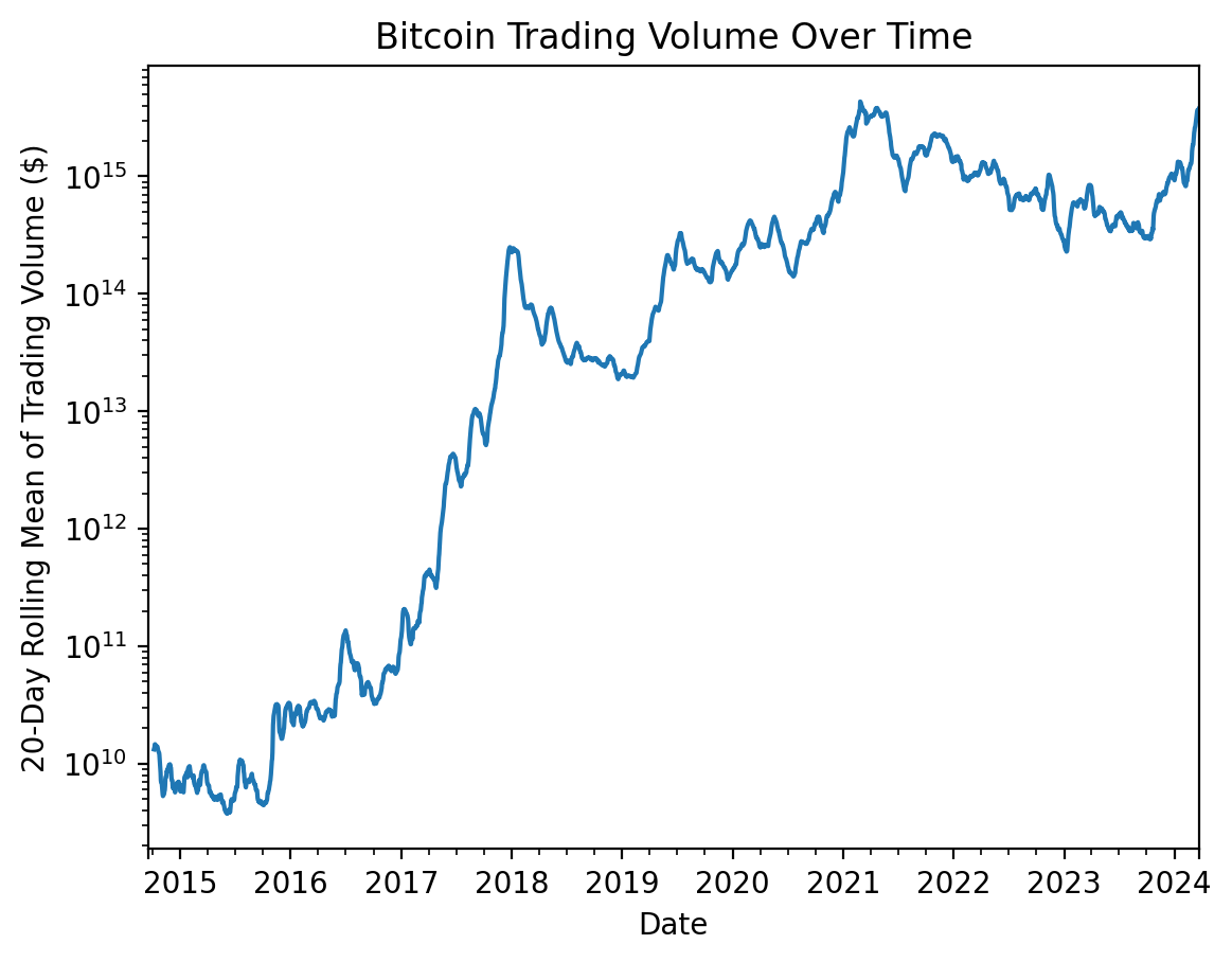
Next, we write a function, since we might want to calculate simple moving averages (SMAs) more than once. The following calc_sma() function accepts:
- A data frame
dfof daily values fromyfinance.download() - An integer
nthat specifies the number of trading days in the SMA window
And returns the original data frame df plus the following columns:
Returnfor the daily returnsSMAfor then-trading-day moving averageSignalfor the weight on the security for each dayStrategyfor the return on the SMA strategy
def calc_sma(df, n):
    return (
        df
        .assign(
            Return=lambda x: x['Adj Close'].pct_change(),
            SMA=lambda x: x['Adj Close'].rolling(n).mean(),
            Signal=lambda x: np.select(
                condlist=[x['Adj Close'].shift(1)>x['SMA'].shift(1), x['Adj Close'].shift(1)<=x['SMA'].shift(1)],
                choicelist=[1, 0],
                default=np.nan
            ),
            Strategy=lambda x: x['Signal'] * x['Return']
        )
    )
Finally, we calculate the SMA(20). We can drop the last row to avoid partial trading-day returns. Recall the last row from yfinance.download() may not be at the close.
btc_sma = btc.iloc[:-1].pipe(calc_sma, n=20)

btc_sma.tail()| Variable | Open | High | Low | Close | Adj Close | Volume | Return | SMA | Signal | Strategy |
|---|---|---|---|---|---|---|---|---|---|---|
| Date | ||||||||||
| 2024-03-17 | 65316.3438 | 68845.7188 | 64545.3164 | 68390.6250 | 68390.6250 | 44716864318 | 0.0471 | 66530.1934 | 0.0000 | 0.0000 |
| 2024-03-18 | 68371.3047 | 68897.1328 | 66594.2266 | 67548.5938 | 67548.5938 | 49261579492 | -0.0123 | 67053.3545 | 1.0000 | -0.0123 |
| 2024-03-19 | 67556.1328 | 68106.9297 | 61536.1797 | 61912.7734 | 61912.7734 | 74215844794 | -0.0834 | 67023.7537 | 1.0000 | -0.0834 |
| 2024-03-20 | 61930.1562 | 68115.2578 | 60807.7852 | 67913.6719 | 67913.6719 | 66792634382 | 0.0969 | 67359.5182 | 0.0000 | 0.0000 |
| 2024-03-21 | 67911.5859 | 68199.9922 | 64580.9180 | 65491.3906 | 65491.3906 | 44480350565 | -0.0357 | 67512.0561 | 1.0000 | -0.0357 |
For Bitcoin, the SMA(20) strategy works well over the full sample!
names_sma = {'Return': 'Buy-And-Hold', 'Strategy': 'SMA(20)'}

_ = (
    btc_sma
    [['Return', 'Strategy']]
    .dropna()
)

(
    _
    .add(1)
    .cumprod()
    .rename_axis(columns='Strategy')
    .rename(columns=names_sma)
    .plot(logy=True)
)
plt.ylabel('Value ($)')
plt.title(f'Value of $1 Invested in Bitcoin Strategies\nat Close on {_.index[0] - pd.offsets.Day(1):%B %d, %Y}')
plt.show()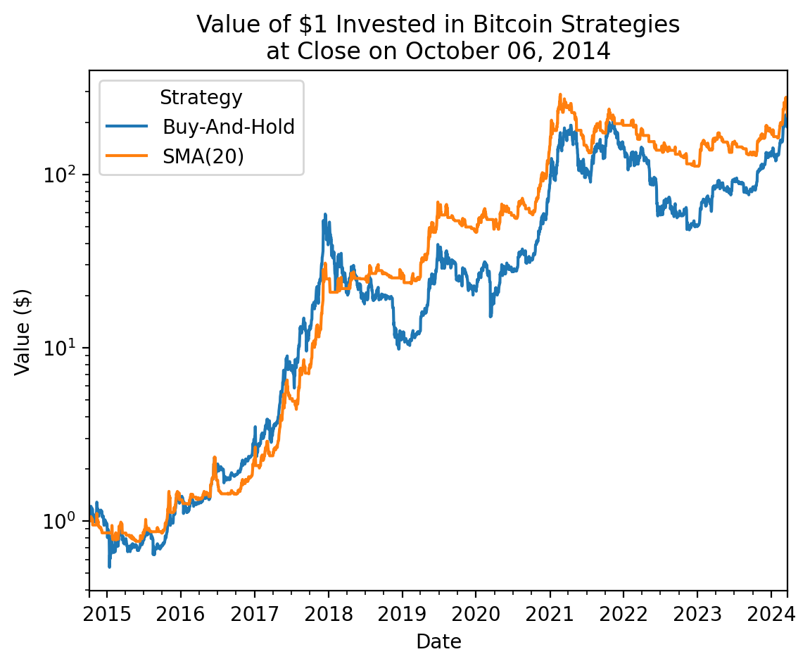
Here are the final values of $1 investments, which are difficult to read on the log scale above.
(
    btc_sma
    [['Return', 'Strategy']]
    .rename_axis(columns='Strategy')
    .rename(columns=names_sma)
    .add(1)
    .prod()
)
Strategy
Buy-And-Hold 143.2025
SMA(20) 217.6557
dtype: float643.2 How does SMA(20) outperform buy-and-hold with this sample?
Consider the following:
- Does SMA(20) avoid the worst performing days? How many of the worst 20 days does SMA(20) avoid? Try the
.sort_values()or.nlargest()method. - Does SMA(20) preferentially avoid low-return days? Try to combine the
.groupby()method andpd.qcut()function. - Does SMA(20) preferentially avoid high-volatility days? Try to combine the
.groupby()method andpd.qcut()function.
The SMA(20) does well here because it avoids 17 of the 20 worst days, without avoiding the best days.
btc_sma.loc[btc_sma['Return'].nsmallest(20).index, ['Signal']].value_counts()Signal
0.0000 17
1.0000 3
Name: count, dtype: int64btc_sma.loc[btc_sma['Return'].nlargest(20).index, ['Signal']].value_counts()Signal
0.0000 10
1.0000 10
Name: count, dtype: int64(
btc_sma
.rename(columns=names_sma)
.groupby('Signal')
[['Buy-And-Hold', 'SMA(20)']]
.describe()
.rename_axis(columns=['Strategy', 'Statistic'])
.stack('Strategy')
)| Statistic | count | mean | std | min | 25% | 50% | 75% | max | |
|---|---|---|---|---|---|---|---|---|---|
| Signal | Strategy | ||||||||
| 0.0000 | Buy-And-Hold | 1542.0000 | 0.0008 | 0.0401 | -0.3717 | -0.0138 | 0.0015 | 0.0163 | 0.2394 |
| SMA(20) | 1542.0000 | 0.0000 | 0.0000 | 0.0000 | 0.0000 | 0.0000 | 0.0000 | 0.0000 | |
| 1.0000 | Buy-And-Hold | 1912.0000 | 0.0034 | 0.0339 | -0.1409 | -0.0112 | 0.0015 | 0.0175 | 0.2525 |
| SMA(20) | 1912.0000 | 0.0034 | 0.0339 | -0.1409 | -0.0112 | 0.0015 | 0.0175 | 0.2525 |
We can also use the seaborn package to visualize Signal (i.e., the portfolio weight on Bitcoin) during periods of high and low Bitcoin returns and volatility. The SMA(20) strategy is long Bitcoin about 55% of the time, with Bitcoin returns are high (bin 2) or low (bin 1).
(
    btc_sma
    [['Return', 'Signal']]
    .dropna()
    .assign(Return_Bin=lambda x: 1 + pd.qcut(x['Return'], q=2, labels=False))
    .pipe(
        sns.barplot,
        x='Return_Bin',
        y='Signal'
    )
)

plt.title('Percentage of Time SMA(20) Strategy is Long Bitcoin\nby Bitcoin Daily Return Bins')
plt.show()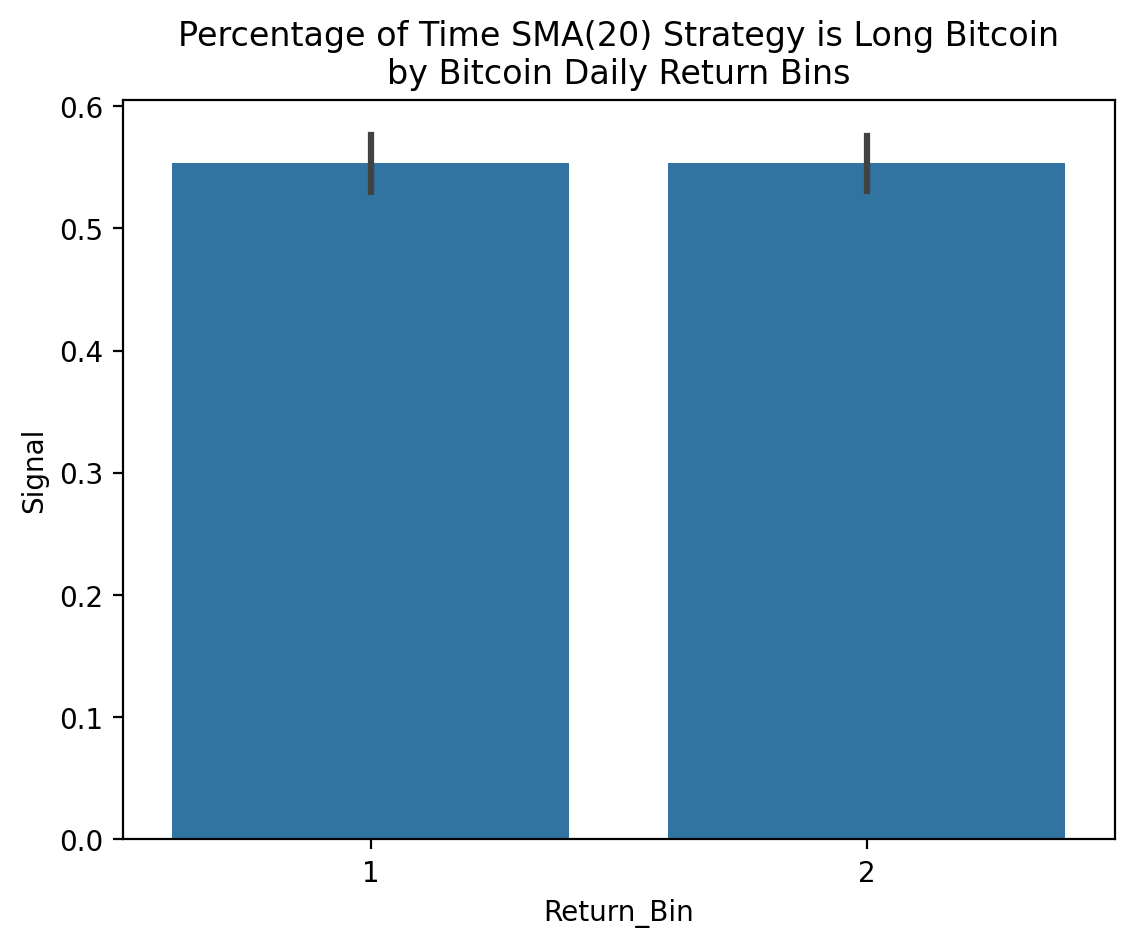
(
    btc_sma
    [['Return', 'Signal']]
    .dropna()
    .assign(Volatility_Bin=lambda x: 1 + pd.qcut(x['Return'].rolling(20).std(), q=2, labels=False))
    .pipe(
        sns.barplot,
        x='Volatility_Bin',
        y='Signal'
    )
)

plt.title('Percentage of Time SMA(20) Strategy is Long Bitcoin\nby Bitcoin 20-Day Volatility Bins')
plt.show()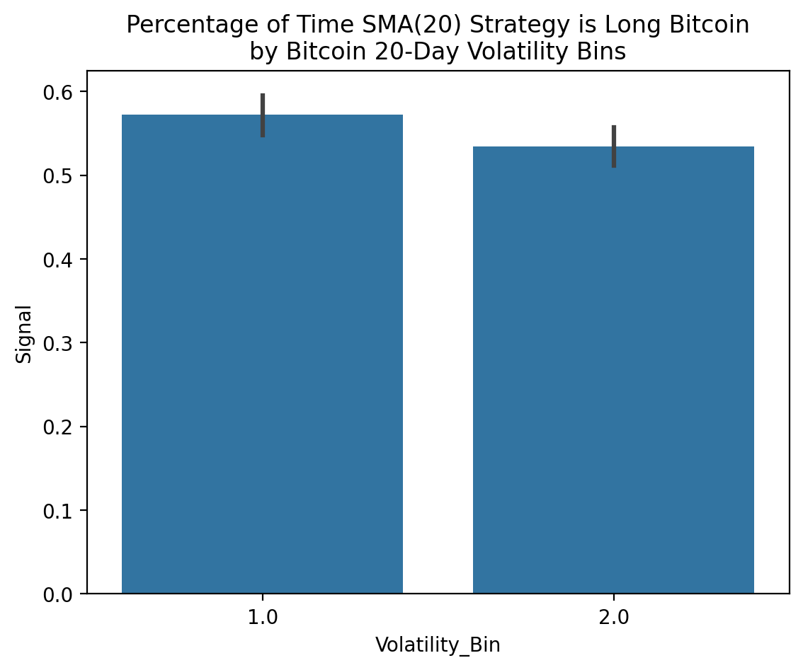
3.3 Implement the SMA(20) strategy with the market factor from French
We need to impute a price before we calculate SMA(20), because French does not provide a price we can use for technical analysis (TA).
ff = (
    pdr.DataReader(
        name='F-F_Research_Data_Factors_daily',
        data_source='famafrench',
        start='1900'
    )
    [0]
    .div(100)
    .assign(
        Mkt=lambda x: x['Mkt-RF'] + x['RF'],
        Price=lambda x: x['Mkt'].add(1).cumprod()
    )
)
C:\Users\r.herron\AppData\Local\Temp\ipykernel_25516\2105953079.py:2: FutureWarning: The argument 'date_parser' is deprecated and will be removed in a future version. Please use 'date_format' instead, or read your data in as 'object' dtype and then call 'to_datetime'.
pdr.DataReader(ff_sma = (
ff
.rename(columns={'Price': 'Adj Close'})
.pipe(calc_sma, n=20)
)
ff_sma.tail()| Mkt-RF | SMB | HML | RF | Mkt | Adj Close | Return | SMA | Signal | Strategy | |
|---|---|---|---|---|---|---|---|---|---|---|
| Date | ||||||||||
| 2024-01-25 | 0.0046 | 0.0004 | 0.0056 | 0.0002 | 0.0048 | 11969.2170 | 0.0048 | 11716.9236 | 1.0000 | 0.0048 |
| 2024-01-26 | -0.0002 | 0.0040 | -0.0027 | 0.0002 | 0.0000 | 11969.4564 | 0.0000 | 11727.1312 | 1.0000 | 0.0000 |
| 2024-01-29 | 0.0085 | 0.0107 | -0.0059 | 0.0002 | 0.0087 | 12073.8301 | 0.0087 | 11742.4928 | 1.0000 | 0.0087 |
| 2024-01-30 | -0.0013 | -0.0126 | 0.0084 | 0.0002 | -0.0011 | 12060.7903 | -0.0011 | 11759.6086 | 1.0000 | -0.0011 |
| 2024-01-31 | -0.0174 | -0.0092 | -0.0030 | 0.0002 | -0.0172 | 11853.5860 | -0.0172 | 11770.3368 | 1.0000 | -0.0172 |
_ = ff_sma[['Return', 'Strategy']].dropna()

(
    _
    .add(1)
    .cumprod()
    .rename_axis(columns='Strategy')
    .rename(columns=names_sma)
    .plot(logy=True)
)
plt.ylabel('Value ($)')
plt.title(f'Value of $1 Invested in Market\nat Close on {_.index[0] - pd.offsets.BDay(1):%B %d, %Y}')
plt.show()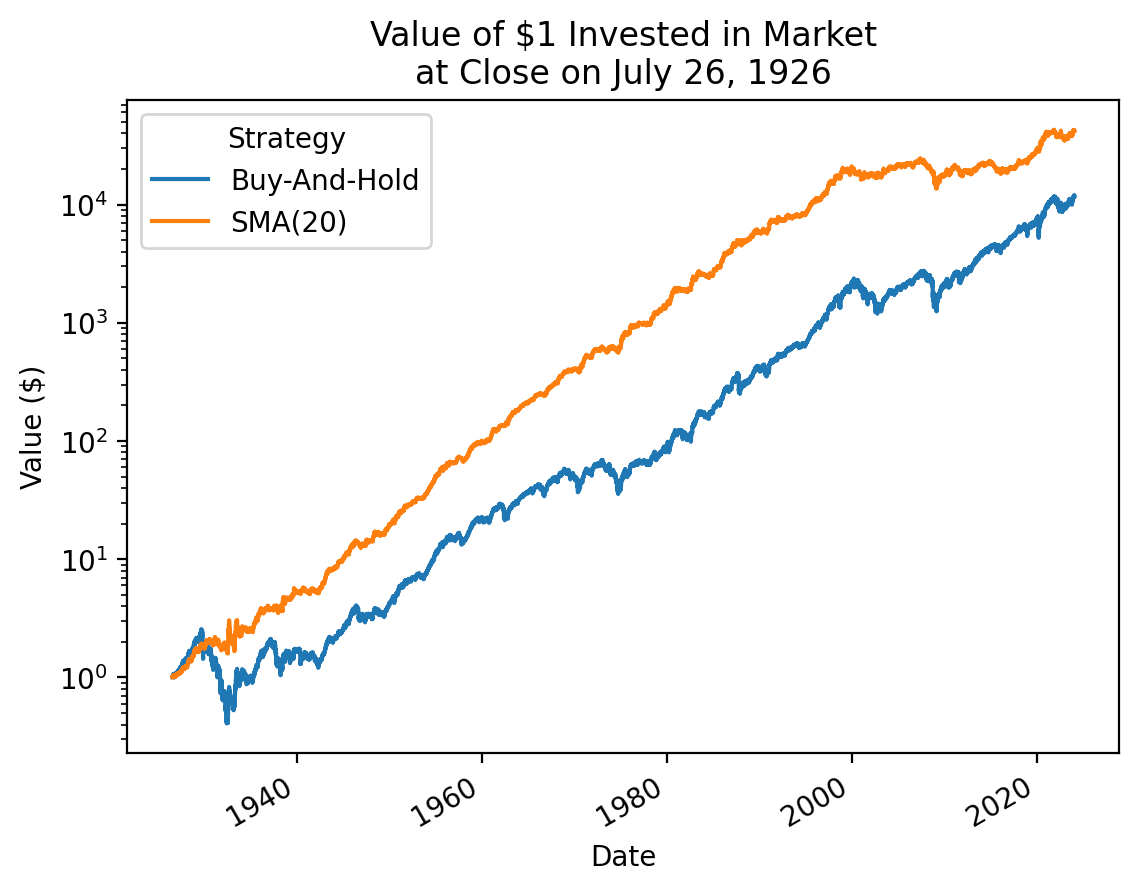
3.4 How often does SMA(20) outperform buy-and-hold with 1-year rolling windows with Bitcoin?
_ = (
    btc_sma
    [['Return', 'Strategy']]
    .pipe(np.log1p)
    .rolling(365)
    .sum()
    .pipe(np.expm1)
)

(
    _
    .dropna()
    .mul(100)
    .rename(columns=names_sma)
    .rename_axis(columns='Strategy')
    .plot()
)

plt.title('One-Year Rolling Returns for Bitcoin')
plt.ylabel('One-Year Rolling Return (%)')

print(
    f'{names_sma['Strategy']} > {names_sma['Return']} for One-Year Rolling Window:',
    (_['Strategy'] > _['Return']).value_counts(),
    sep='\n'
)
SMA(20) > Buy-And-Hold for One-Year Rolling Window:
False 2111
True 1363
Name: count, dtype: int64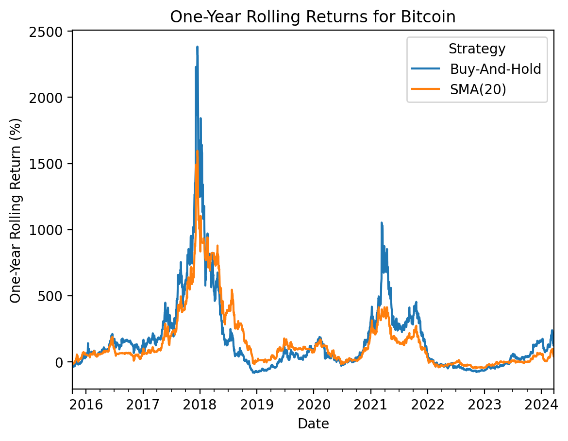
3.5 Implement a long-only BB(20, 2) strategy with Bitcoin
More on Bollinger Bands here and here. In short, Bollinger Bands are bands around a trend, typically defined in terms of simple moving averages and volatilities. Here, long-only BB(20, 2) implies we have upper and lower bands at 2 standard deviations above and below SMA(20):
- Buy when the closing price crosses LB(20) from below, where LB(20) is SMA(20) minus 2 sigma
- Sell when the closing price crosses UB(20) from above, where UB(20) is SMA(20) plus 2 sigma
- No short-selling
The long-only BB(20, 2) is more difficult to implement than the long-only SMA(20) because we need to track buys and sells. For example, if the closing price is between LB(20) and BB(20), we need to know if our last trade was a buy or a sell. Further, if the closing price is below LB(20), we can still be long because we sell when the closing price crosses UB(20) from above.
Here is a function to calculate Bolling Bands and implement the strategy.
def calc_bb(df, m, n):
    return (
        btc
        .assign(
            Return=lambda x: x['Adj Close'].pct_change(),
            SMA=lambda x: x['Adj Close'].rolling(m).mean(), # m-day simple moving averge
            SMV=lambda x: x['Adj Close'].rolling(m).std(), # m-day simple moving volatility
            LB=lambda x: x['SMA'] - n*x['SMV'], # lower band is SMA - n*SMV
            UB=lambda x: x['SMA'] + n*x['SMV'], # upper band is SMA + n*SMV
            Signal_with_nan=lambda x: np.select(
                condlist=[
                    # long when price>LB yesterday but price<=LB two days ago
                    (x['Adj Close'].shift(1)>x['LB'].shift(1)) & (x['Adj Close'].shift(2)<=x['LB'].shift(2)),
                    # neutral when price<UB yesterday but price>=UB two days ago
                    (x['Adj Close'].shift(1)<x['UB'].shift(1)) & (x['Adj Close'].shift(2)>=x['UB'].shift(2)),
                ],
                choicelist=[
                    1,
                    0
                ],
                default=np.nan
            ),
            Signal=lambda x: x['Signal_with_nan'].ffill(), # carryforward last trade decisions
            Strategy=lambda x: x['Signal'] * x['Return']
        )
    )
Again, we drop the last day to omit partial returns.
btc_bb = btc.iloc[:-1].pipe(calc_bb, m=20, n=2)

btc_bb.tail()| Variable | Open | High | Low | Close | Adj Close | Volume | Return | SMA | SMV | LB | UB | Signal_with_nan | Signal | Strategy |
|---|---|---|---|---|---|---|---|---|---|---|---|---|---|---|
| Date | ||||||||||||||
| 2024-03-18 | 68371.3047 | 68897.1328 | 66594.2266 | 67548.5938 | 67548.5938 | 49261579492 | -0.0123 | 67053.3545 | 3615.2985 | 59822.7575 | 74283.9515 | NaN | 0.0000 | -0.0000 |
| 2024-03-19 | 67556.1328 | 68106.9297 | 61536.1797 | 61912.7734 | 61912.7734 | 74215844794 | -0.0834 | 67023.7537 | 3656.6873 | 59710.3790 | 74337.1284 | NaN | 0.0000 | -0.0000 |
| 2024-03-20 | 61930.1562 | 68115.2578 | 60807.7852 | 67913.6719 | 67913.6719 | 66792634382 | 0.0969 | 67359.5182 | 3392.3919 | 60574.7343 | 74144.3020 | NaN | 0.0000 | 0.0000 |
| 2024-03-21 | 67911.5859 | 68199.9922 | 64580.9180 | 65491.3906 | 65491.3906 | 44480350565 | -0.0357 | 67512.0561 | 3223.9829 | 61064.0903 | 73960.0218 | NaN | 0.0000 | -0.0000 |
| 2024-03-22 | 65492.0781 | 66613.6719 | 62865.6641 | 62865.6641 | 62865.6641 | 42267766784 | -0.0401 | 67553.8469 | 3153.8337 | 61246.1795 | 73861.5142 | NaN | 0.0000 | -0.0000 |
names_bb = {'Return': 'Buy-And-Hold', 'Strategy': 'BB(20, 2)'}

_ = (
    btc_bb
    [['Return', 'Strategy']]
    .dropna()
)

(
    _
    .add(1)
    .cumprod()
    .rename_axis(columns='Strategy')
    .rename(columns=names_bb)
    .plot(logy=True)
)
plt.ylabel('Value ($)')
plt.title(f'Value of $1 Invested in Bitcoin\nat Close on {_.index[0] - pd.offsets.Day(1):%B %d, %Y}')
plt.show()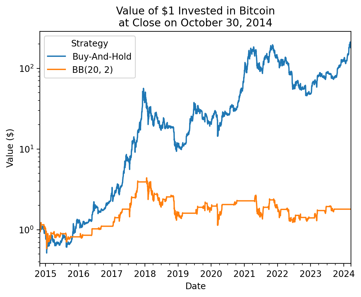
Here are the final values of $1 investments, which are difficult to read on the log scale above.
(
    btc_bb
    [['Return', 'Strategy']]
    .rename(columns=names_bb)
    .rename_axis(columns='Strategy')
    .add(1)
    .prod()
)
Strategy
Buy-And-Hold 137.4612
BB(20, 2) 1.8011
dtype: float64It might be helpful to plot a few months of Bitcoin prices and signals to better understand the BB(20, 2) strategy
fig, ax = plt.subplots(nrows=2, ncols=1, sharex=True)
_ = btc_bb.loc['2023-02':'2023-03']

ax[0].plot(_[['Adj Close']], label='Price')
ax[0].plot(_[['SMA']], label='SMA(20)')
ax[0].plot(_[['UB']], label='LB and UB', color='green', linestyle=':')
ax[0].plot(_[['LB']], color='green', linestyle=':')
ax[0].legend()
ax[0].set_ylabel('Price ($)')

ax[1].plot(_[['Signal']], label='Signal')
ax[1].legend()
ax[1].set_ylabel('Signal')

ax[0].yaxis.set_major_formatter(ticker.StrMethodFormatter('{x:,.0f}'))
fig.autofmt_xdate()

plt.suptitle('Key Variables in Bitcoin BB(20, 2) Strategy')
plt.show()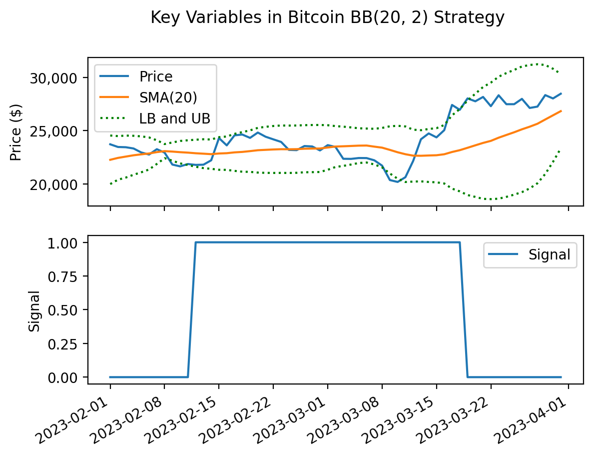
3.6 Implement a long-short RSI(14) strategy with Bitcoin
From Fidelity:
The Relative Strength Index (RSI), developed by J. Welles Wilder, is a momentum oscillator that measures the speed and change of price movements. The RSI oscillates between zero and 100. Traditionally the RSI is considered overbought when above 70 and oversold when below 30. Signals can be generated by looking for divergences and failure swings. RSI can also be used to identify the general trend.
Here is the RSI formula: \(RSI(n) = 100 - \frac{100}{1 + RS(n)}\), where \(RS(n) = \frac{SMA(U, n)}{SMA(D, n)}\). For “up days”, \(U = \Delta Adj\ Close\) and \(D = 0\), and, for “down days”, \(U = 0\) and \(D = - \Delta Adj\ Close\). Therefore, \(U\) and \(D\) are always non-negative. We can learn more about RSI here.
We will implement a long-short RSI(14) as follows:
- Enter a long position when the RSI crosses 30 from below, and exit the position when the RSI crosses 50 from below
- Enter a short position when the RSI crosses 70 from above, and exit the position when the RSI crosses 50 from above
def calc_rsi(df, n, lb, mb, ub):
    return df.assign(
        Return=lambda x: x['Adj Close'].pct_change(),
        Diff=lambda x: x['Adj Close'].diff(),
        U=lambda x: np.select(
            condlist=[x['Diff'] >= 0, x['Diff'] < 0],
            choicelist=[x['Diff'], 0],
            default=np.nan
        ),
        D=lambda x: np.select(
            condlist=[x['Diff'] <= 0, x['Diff'] > 0],
            choicelist=[-1 * x['Diff'], 0],
            default=np.nan
        ),
        SMAU=lambda x: x['U'].rolling(n).mean(),
        SMAD=lambda x: x['D'].rolling(n).mean(),
        RS=lambda x: x['SMAU'] / x['SMAD'],
        RSI=lambda x: 100 - 100 / (1 + x['RS']),
        Signal_with_nan = lambda x: np.select(
            condlist=[
                (x['RSI'].shift(1) >= lb) & (x['RSI'].shift(2) < lb),
                (x['RSI'].shift(1) >= mb) & (x['RSI'].shift(2) < mb),
                (x['RSI'].shift(1) <= ub) & (x['RSI'].shift(2) > ub),
                (x['RSI'].shift(1) <= mb) & (x['RSI'].shift(2) > mb),
            ],
            choicelist=[
                1,
                0,
                -1,
                0
            ],
            default=np.nan
        ),
        Signal=lambda x: x['Signal_with_nan'].ffill(),
        Strategy=lambda x: x['Signal'] * x['Return']
    )
Again, we drop the last day to omit partial returns.
btc_rsi = btc.iloc[:-1].pipe(calc_rsi, n=14, mb=2, lb=30, ub=70)

btc_rsi.tail()| Variable | Open | High | Low | Close | Adj Close | Volume | Return | Diff | U | D | SMAU | SMAD | RS | RSI | Signal_with_nan | Signal | Strategy |
|---|---|---|---|---|---|---|---|---|---|---|---|---|---|---|---|---|---|
| Date | |||||||||||||||||
| 2024-03-17 | 65316.3438 | 68845.7188 | 64545.3164 | 68390.6250 | 68390.6250 | 44716864318 | 0.0471 | 3075.5078 | 3075.5078 | 0.0000 | 1297.3906 | 924.3011 | 1.4036 | 58.3965 | NaN | -1.0000 | -0.0471 |
| 2024-03-18 | 68371.3047 | 68897.1328 | 66594.2266 | 67548.5938 | 67548.5938 | 49261579492 | -0.0123 | -842.0312 | 0.0000 | 842.0312 | 928.6018 | 984.4461 | 0.9433 | 48.5404 | NaN | -1.0000 | 0.0123 |
| 2024-03-19 | 67556.1328 | 68106.9297 | 61536.1797 | 61912.7734 | 61912.7734 | 74215844794 | -0.0834 | -5635.8203 | 0.0000 | 5635.8203 | 928.6018 | 1063.4894 | 0.8732 | 46.6144 | NaN | -1.0000 | 0.0834 |
| 2024-03-20 | 61930.1562 | 68115.2578 | 60807.7852 | 67913.6719 | 67913.6719 | 66792634382 | 0.0969 | 6000.8984 | 6000.8984 | 0.0000 | 1192.5513 | 1063.4894 | 1.1214 | 52.8604 | NaN | -1.0000 | -0.0969 |
| 2024-03-21 | 67911.5859 | 68199.9922 | 64580.9180 | 65491.3906 | 65491.3906 | 44480350565 | -0.0357 | -2422.2812 | 0.0000 | 2422.2812 | 1134.0742 | 1236.5095 | 0.9172 | 47.8395 | NaN | -1.0000 | 0.0357 |
names_rsi = {'Return': 'Buy-And-Hold', 'Strategy': 'RSI(14)'}

_ = btc_rsi[['Return', 'Strategy']].dropna()

(
    _
    .add(1)
    .cumprod()
    .rename_axis(columns='Strategy')
    .rename(columns=names_rsi)
    .plot(logy=True)
)

plt.ylabel('Value ($)')
plt.title(f'Value of $1 Invested in Bitcoin Strategies\nat Close on {_.index[0] - pd.offsets.Day(1):%B %d, %Y}')
plt.show()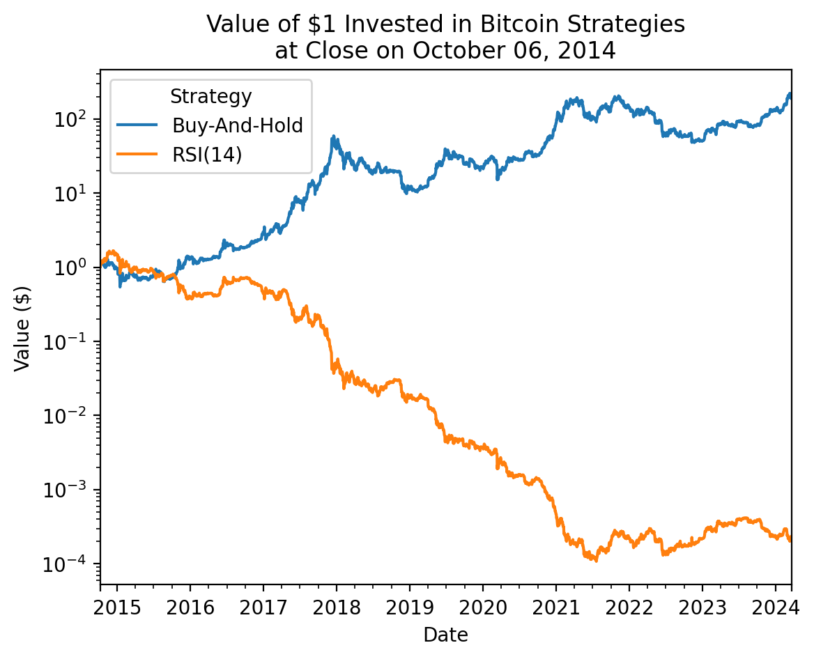
Here are the final values of $1 investments, which are difficult to read on the log scale above.
(
    btc_rsi
    [['Return', 'Strategy']]
    .rename(columns=names_sma)
    .rename_axis(columns='Strategy')
    .add(1)
    .prod()
)
Strategy
Buy-And-Hold 143.2025
SMA(20) 0.0002
dtype: float64Shorting Bitcoin has been dangerous!
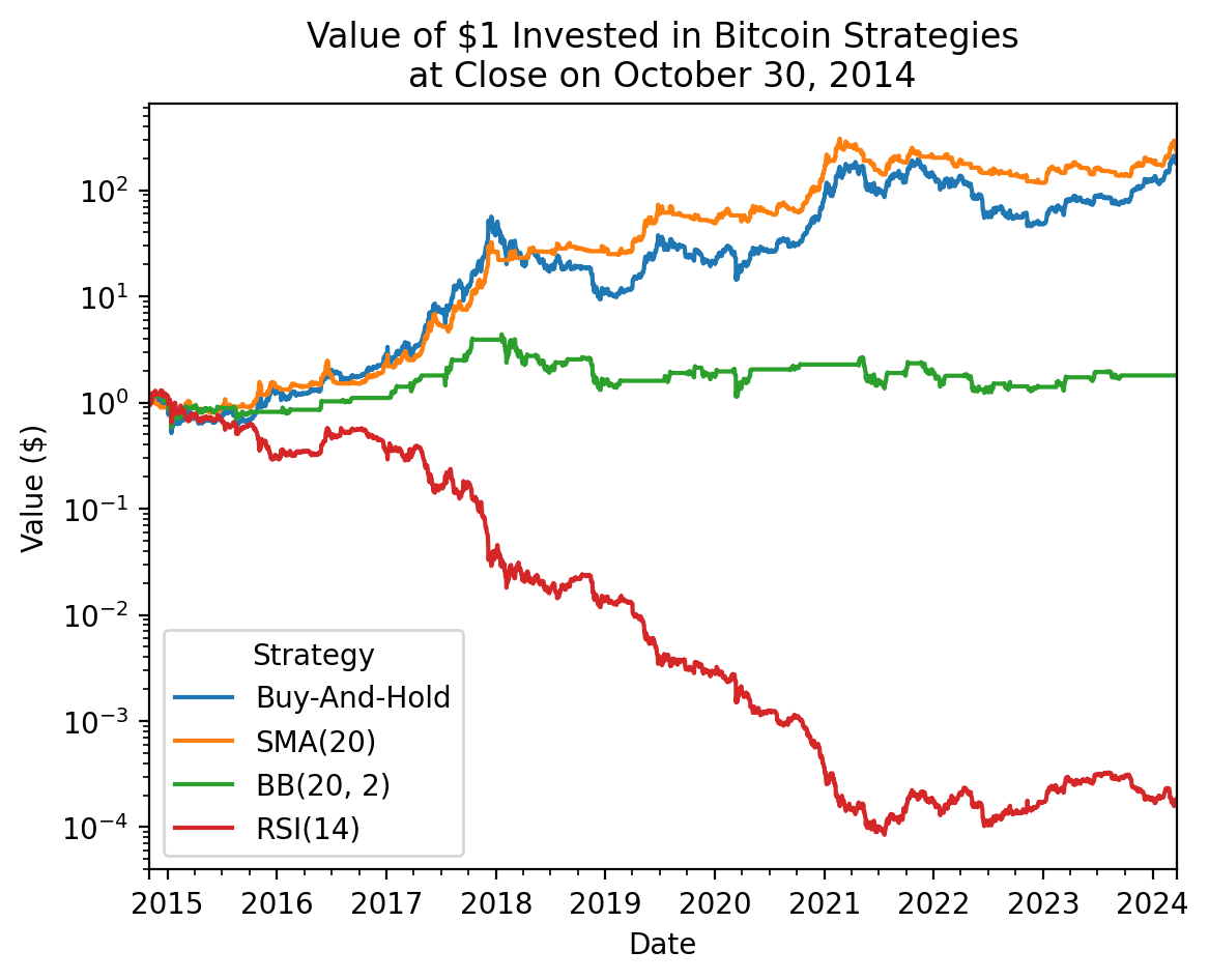
We can compare all three TA strategies!
_ = (
    btc_sma[['Return', 'Strategy']]
    .join(
        btc_bb[['Strategy']].add_suffix('_BB'),
    )
    .join(
        btc_rsi[['Strategy']].add_suffix('_RSI'),
    )
    .dropna()
)


(
    _
    .add(1)
    .cumprod()
    .rename_axis(columns='Strategy')
    .rename(columns=
            {
                'Return': 'Buy-And-Hold',
                'Strategy': 'SMA(20)',
                'Strategy_BB': 'BB(20, 2)',
                'Strategy_RSI': 'RSI(14)',
            }
           )
    .plot(logy=True)
)

plt.ylabel('Value ($)')
plt.title(f'Value of $1 Invested in Bitcoin Strategies\nat Close on {_.index[0] - pd.offsets.Day(1):%B %d, %Y}')
plt.show()