import matplotlib.pyplot as plt
import numpy as np
import pandas as pd
import pandas_datareader as pdr
import scipy.optimize as sco
import yfinance as yfHerron Topic 4 - Practice for Section 03
FINA 6333 for Spring 2024
1 Announcements
- This week:
- Tuesday: Herron Topic 4 on portfolio optimization
- Thursday and Friday: MSFQ assessment exam in your scheduled classroom and time
- Next week: Group work on Project 3 all week
- Last week:
- Tuesday: Project 3 due at 11:59 PM on Tuesday, 4/23
- Thursday and Friday: Office hours during class time
2 10-Minute Recap
Pease review the lecture notebook, which provides a streamlined introduction to optimization in Python!
3 Practice
%precision 4
pd.options.display.float_format = '{:.4f}'.format
%config InlineBackend.figure_format = 'retina'
3.1 Find the maximum Sharpe Ratio portfolio of MATANA stocks over the last three years
Note that sco.minimize() finds minimums, so you need to minimize the negative Sharpe Ratio.
matana = (
    yf.download(tickers='META AAPL TSLA AMZN NVDA GOOG')
    ['Adj Close']
    .iloc[:-1]
    .pct_change()
)
[*********************100%%**********************] 6 of 6 completedff = (
pdr.DataReader(
name='F-F_Research_Data_Factors_daily',
data_source='famafrench',
start='1900'
)
[0]
.div(100)
)C:\Users\r.herron\AppData\Local\Temp\ipykernel_9456\2049483829.py:2: FutureWarning: The argument 'date_parser' is deprecated and will be removed in a future version. Please use 'date_format' instead, or read your data in as 'object' dtype and then call 'to_datetime'.
pdr.DataReader(def calc_sharpe(x, r, tgt, ppy):
rp = r.dot(x)
rp_tgt = rp.sub(tgt)
return np.sqrt(ppy) * rp_tgt.mean() / rp_tgt.std()def calc_neg_sharpe(x, r, tgt, ppy):
return -1 * calc_sharpe(x=x, r=r, tgt=tgt, ppy=ppy)After class, I decided to write a get_equal_weights() function to easily calculate \(\frac{1}{n}\) portfolio weights.
def get_equal_weights(r):
    n = r.shape[1]
    return np.ones(n) / n
x0 = get_equal_weights(r=matana)
x0array([0.1667, 0.1667, 0.1667, 0.1667, 0.1667, 0.1667])We can test our function!
calc_sharpe(
    x=x0,
    r=matana.loc['2021':'2023'],
    tgt=ff['RF'],
    ppy=252
)0.6336rp_tgt = matana.loc['2021':'2023'].dot(x0).sub(ff['RF'])
np.sqrt(252) * rp_tgt.mean() / rp_tgt.std()0.6336calc_neg_sharpe(
x=x0,
r=matana.loc['2021':'2023'],
tgt=ff['RF'],
ppy=252
)-0.6336res_sr = sco.minimize(
fun=calc_neg_sharpe,
x0=matana.pipe(get_equal_weights),
args=(matana.loc['2021':'2023'], ff['RF'], 252),
bounds=((0, 1) for c in matana.columns),
constraints=(
{'type':'eq', 'fun': lambda x: x.sum() - 1} # eq constraint met when equal to zero
)
)
res_sr message: Optimization terminated successfully
success: True
status: 0
fun: -1.0660861120691252
x: [ 4.957e-17 0.000e+00 0.000e+00 3.409e-17 1.000e+00
7.178e-17]
nit: 5
jac: [ 3.206e-02 3.530e-01 -1.079e-02 1.151e-01 -3.910e-02
2.773e-01]
nfev: 35
njev: 5plt.barh(
y=matana.columns,
width=res_sr['x']
)
plt.ylabel('Ticker')
plt.xlabel('Portfolio Weight')
plt.title('Maximum Sharpe Ratio Portfolio Weights\n for MATANA Stocks from 2021 through 2023')
plt.show()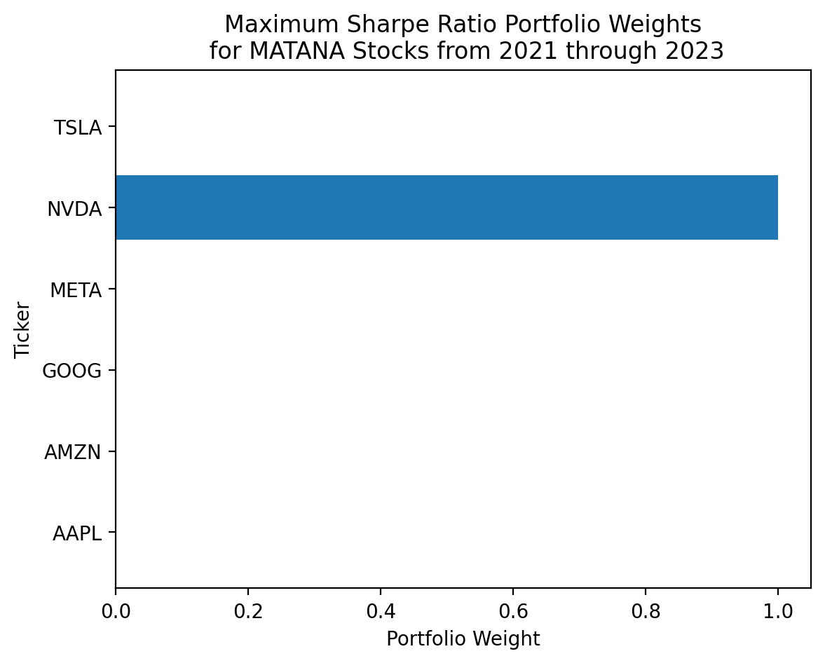
3.2 Find the maximum Sharpe Ratio portfolio of MATANA stocks over the last three years, but allow short weights up to 10% on each stock
res_sr_2 = sco.minimize(
    fun=calc_neg_sharpe,
    x0=matana.pipe(get_equal_weights),
    args=(matana.loc['2021':'2023'], ff['RF'], 252),
    bounds=((-0.1, 1.5) for c in matana.columns),
    constraints=(
        {'type':'eq', 'fun': lambda x: x.sum() - 1} # eq constraint met when equal to zero
    )
)

res_sr_2
message: Optimization terminated successfully
success: True
status: 0
fun: -1.13530096310489
x: [-1.000e-01 -1.000e-01 2.348e-01 -1.000e-01 1.165e+00
-1.000e-01]
nit: 6
jac: [ 2.074e-02 3.100e-01 1.634e-02 7.954e-02 1.697e-02
1.877e-01]
nfev: 42
njev: 6(
pd.DataFrame(
data={
'Long Only': res_sr['x'],
'Short up to 10% per Stock': res_sr_2['x']
},
index=matana.columns
)
.plot(kind='barh')
)
plt.ylabel('Ticker')
plt.xlabel('Portfolio Weight')
plt.title('Maximum Sharpe Ratio Portfolio Weights\n for MATANA Stocks from 2021 through 2023')
plt.show()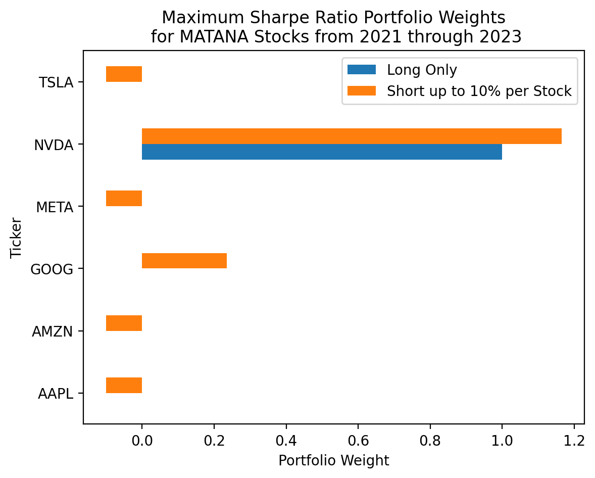
By relaxing the long-only constrain (via changes to bounds=), the weights on AAPL, AMZN, META, and TSLA go from zero to -10%. Also, the Sharpe Ratio increases because we relax a binding constraint.
calc_sharpe(
    x=res_sr['x'],
    r=matana.loc['2021':'2023'],
    tgt=ff['RF'],
    ppy=252
)1.0661calc_sharpe(
x=res_sr_2['x'],
r=matana.loc['2021':'2023'],
tgt=ff['RF'],
ppy=252
)1.13533.3 Find the maximum Sharpe Ratio portfolio of MATANA stocks over the last three years, but allow total short weights of up to 30%
Now we need an inequality constraint! We will use an inequality constraint to make sure the sum of the negative portfolio weights is greater than \(-0.3\).
x = np.arange(6) - 3
xarray([-3, -2, -1, 0, 1, 2])We do this by:
- Slicing the negative weights in
xwithx[x < 0] - Constraining the sum of these negative weights to be \(\geq -0.3\), which is met when
x[x < 0].sum() + 0.3is non-negative.
res_sr_3 = sco.minimize(
fun=calc_neg_sharpe,
x0=matana.pipe(get_equal_weights),
args=(matana.loc['2021':'2023'], ff['RF'], 252),
bounds=((-0.3, 1.3) for c in matana.columns),
constraints=(
{'type':'eq', 'fun': lambda x: x.sum() - 1}, # eq constraint met when = 0
{'type':'ineq', 'fun': lambda x: x[x < 0].sum() + 0.3} # ineq constraint met when >= 0
)
)
res_sr_3C:\Users\r.herron\AppData\Local\miniconda3\envs\fina6333\Lib\site-packages\scipy\optimize\_optimize.py:404: RuntimeWarning: Values in x were outside bounds during a minimize step, clipping to bounds
warnings.warn("Values in x were outside bounds during a " message: Optimization terminated successfully
success: True
status: 0
fun: -1.1616529795363868
x: [ 5.476e-07 -3.000e-01 2.717e-01 -2.773e-08 1.028e+00
-2.239e-05]
nit: 43
jac: [ 5.523e-02 3.113e-01 4.328e-02 1.434e-01 4.188e-02
3.028e-01]
nfev: 471
njev: 43(
pd.DataFrame(
data={
'Long Only': res_sr['x'],
'Short up to 10% per Stock': res_sr_2['x'],
'Short up to 30% Total': res_sr_3['x']
},
index=matana.columns
)
.plot(kind='barh')
)
plt.ylabel('Ticker')
plt.xlabel('Portfolio Weight')
plt.title('Maximum Sharpe Ratio Portfolio Weights\n for MATANA Stocks from 2021 through 2023')
plt.show()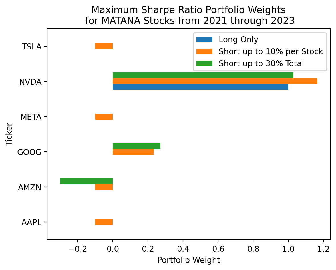
The Sharpe Ratio is higher here than in the previous exercise, but this will not always be the case because we relax slightly different constraints. That is, here we allow up to 30% short in one stock, but only allow up to 30% short across all stocks. In the previous example, we only allow up to 10% short in each stock, but allow up to 50% short across all stocks.
calc_sharpe(
    x=res_sr_2['x'],
    r=matana.loc['2021':'2023'],
    tgt=ff['RF'],
    ppy=252
)1.1353calc_sharpe(
x=res_sr_3['x'],
r=matana.loc['2021':'2023'],
tgt=ff['RF'],
ppy=252
)1.16173.4 Find the maximum Sharpe Ratio portfolio of MATANA stocks over the last three years, but do not allow any weight to exceed 30% in magnitude
res_sr_4 = sco.minimize(
    fun=calc_neg_sharpe,
    x0=matana.pipe(get_equal_weights),
    args=(matana.loc['2021':'2023'], ff['RF'], 252),
    bounds=((0, 0.3) for c in matana.columns),
    constraints=(
        {'type':'eq', 'fun': lambda x: x.sum() - 1}, # eq constraint met when = 0
    )
)

res_sr_4
message: Optimization terminated successfully
success: True
status: 0
fun: -0.8830355215983107
x: [ 3.000e-01 0.000e+00 3.000e-01 1.000e-01 3.000e-01
9.194e-17]
nit: 3
jac: [ 1.089e-01 5.852e-01 8.385e-02 3.099e-01 -5.076e-01
3.305e-01]
nfev: 21
njev: 3(
pd.DataFrame(
data={
'Long Only': res_sr['x'],
'Short up to 10% per Stock': res_sr_2['x'],
'Short up to 30% Total': res_sr_3['x'],
'Long Only up to 30% per Stock': res_sr_4['x']
},
index=matana.columns
)
.plot(kind='barh')
)
plt.ylabel('Ticker')
plt.xlabel('Portfolio Weight')
plt.title('Maximum Sharpe Ratio Portfolio Weights\n for MATANA Stocks from 2021 through 2023')
plt.show()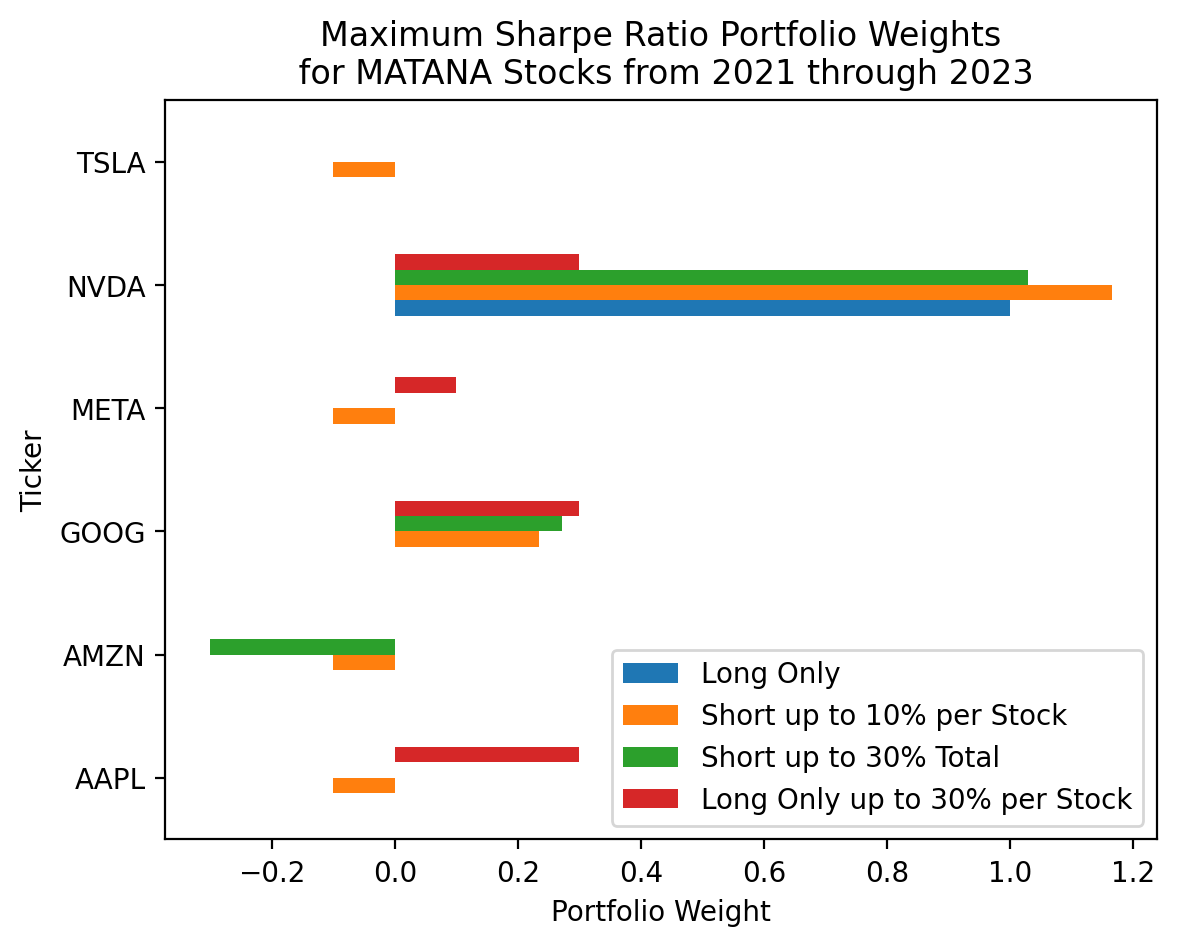
3.5 Find the minimum 95% Value at Risk (Var) portfolio of MATANA stocks over the last three years
More on VaR here.
def calc_var(x, r, q):
    return r.dot(x).quantile(q)
def calc_neg_var(x, r, q):
return -1 * calc_var(x=x, r=r, q=q)res_var = sco.minimize(
fun=calc_neg_var,
x0=matana.pipe(get_equal_weights),
args=(matana.loc['2021':'2023'], 0.05),
bounds=[(0,1) for c in matana],
constraints=(
{'type': 'eq', 'fun': lambda x: x.sum() - 1}, # minimize drives "eq" constraints to zero
)
)
res_var message: Optimization terminated successfully
success: True
status: 0
fun: 0.032516573438853356
x: [ 2.102e-01 1.989e-01 2.292e-01 1.593e-01 2.788e-17
2.024e-01]
nit: 7
jac: [ 3.662e-02 2.644e-02 2.760e-02 2.072e-02 3.928e-02
4.908e-02]
nfev: 61
njev: 7calc_var(x=res_var['x'], r=matana.loc['2021':'2023'], q=0.05)-0.0325plt.barh(
y=matana.columns,
width=res_var['x']
)
plt.ylabel('Ticker')
plt.xlabel('Portfolio Weight')
plt.title('Minimum 5% Value at Risk Portfolio Weights\n for MATANA Stocks from 2021 through 2023')
plt.show()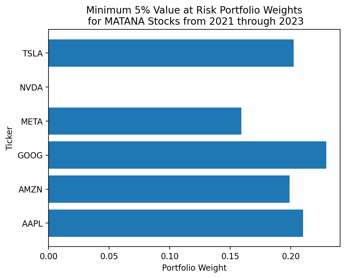
3.6 Find the minimum maximum draw down portfolio of MATANA stocks over the last three years
def calc_max_dd(x, r):
    rp = r.dot(x)
    pp = rp.add(1).cumprod()
    cummax = pp.cummax()
    dd = (cummax - pp) / cummax
    return dd.max()
res_dd = sco.minimize(
fun=calc_max_dd,
x0=matana.pipe(get_equal_weights),
args=(matana.loc['2021':'2023'],),
bounds=[(0,1) for c in matana.columns],
constraints=(
{'type': 'eq', 'fun': lambda x: x.sum() - 1}, # minimize drives "eq" constraints to zero
)
)
res_dd message: Optimization terminated successfully
success: True
status: 0
fun: 0.3091281528292103
x: [ 1.000e+00 0.000e+00 0.000e+00 0.000e+00 0.000e+00
0.000e+00]
nit: 6
jac: [ 2.995e-01 4.945e-01 3.778e-01 6.189e-01 4.966e-01
8.402e-01]
nfev: 42
njev: 6plt.barh(
y=matana.columns,
width=res_dd['x']
)
plt.ylabel('Ticker')
plt.xlabel('Portfolio Weight')
plt.title('Minimum Maximum Draw Down Portfolio Weights\n for MATANA Stocks from 2021 through 2023')
plt.show()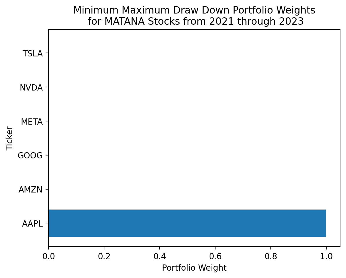
3.7 Find the minimum maximum draw down portfolio with all available data for the current Dow-Jones Industrial Average (DJIA) stocks
You can find the DJIA tickers on Wikipedia.
tickers = pd.read_html('https://en.wikipedia.org/wiki/Dow_Jones_Industrial_Average')[1]['Symbol'].to_list()djia = (
yf.download(tickers=tickers)
['Adj Close']
.iloc[:-1]
.pct_change()
)[*********************100%%**********************] 30 of 30 completedres_dd_2 = sco.minimize(
fun=calc_max_dd,
x0=djia.pipe(get_equal_weights),
args=(djia.loc['2021':'2023'],),
bounds=[(0,1) for c in djia.columns],
constraints=(
{'type': 'eq', 'fun': lambda x: x.sum() - 1}, # minimize drives "eq" constraints to zero
)
)
res_dd_2 message: Optimization terminated successfully
success: True
status: 0
fun: 0.07659155782931011
x: [ 4.176e-02 1.931e-02 ... 1.780e-02 4.305e-02]
nit: 35
jac: [-2.237e-02 1.809e-01 ... 4.256e-02 9.220e-02]
nfev: 1140
njev: 35plt.barh(
y=djia.columns,
width=res_dd_2['x']
)
plt.ylabel('Ticker')
plt.xlabel('Portfolio Weight')
plt.title('Minimum Maximum Draw Down Portfolio Weights\n for DJIA Stocks from 2021 through 2023'
)
plt.show()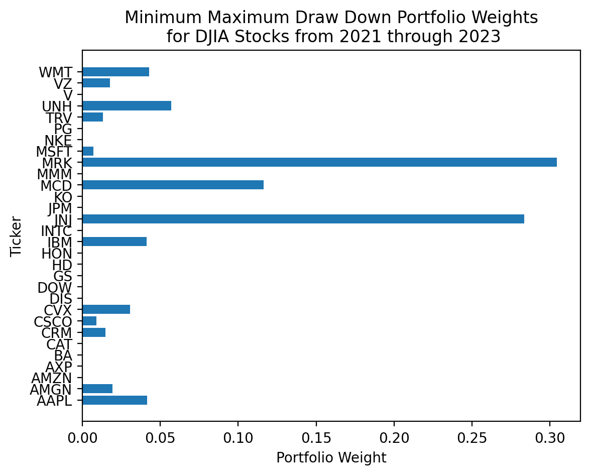
3.8 Plot the (mean-variance) efficient frontier with all available data for the current the DJIA stocks
The range of target returns in tret span from the minimum to the maximum mean single-stock returns. We will loop over these target returns, finding the minimum variance portfolio for each target return.
_ = djia.loc['2021':'2023'].mean().mul(252)
tret = np.linspace(_.min(), _.max(), 25)
def calc_vol(x, r, ppy):
return np.sqrt(ppy) * r.dot(x).std()def calc_mean(x, r, ppy):
return ppy * r.dot(x).mean()res_ef = []
for t in tret:
_ = sco.minimize(
fun=calc_vol, # minimize portfolio volatility
x0=djia.pipe(get_equal_weights), # initial portfolio weights
args=(djia.loc['2021':'2023'], 252), # additional arguments to fun, in order
bounds=((0, 1) for c in djia.columns), # bounds limit the search space for each portfolio weight
constraints=(
{'type': 'eq', 'fun': lambda x: x.sum() - 1}, # constrain sum of weights to one
{
'type': 'eq',
'fun': lambda x: calc_mean(x=x, r=djia.loc['2021':'2023'], ppy=252) - t
} # constrains portfolio mean return to the target return
)
)
res_ef.append(_)List res_ef contains the results of all 25 minimum-variance portfolios. For example, res_ef[0] is the minimum variance portfolio for the lowest target return.
res_ef[0] message: Optimization terminated successfully
success: True
status: 0
fun: 0.29954840655072656
x: [ 2.359e-16 0.000e+00 ... 2.418e-09 0.000e+00]
nit: 2
jac: [ 1.253e-01 3.352e-02 ... 4.880e-02 4.303e-02]
nfev: 62
njev: 2I typically check that all portfolio volatility minimization succeeds. If a portfolio volatility minimization fails, we should check our function, bounds, and constraints.
for r in res_ef:
    assert r['success']
We can combine the target returns and volatilities into a data frame ef.
ef = pd.DataFrame(
    {
        'tret': tret,
        'tvol': [r['fun'] if r['success'] else np.nan for r in res_ef]
    }
)ef.mul(100).plot(x='tvol', y='tret', legend=False)
plt.ylabel('Annualized Mean Return (%)')
plt.xlabel('Annualized Volatility (%)')
plt.title('Mean-Variance Efficient Frontier\nfor DJIA Stocks from 2021 through 2023')
for t, x, y in zip(
djia.columns,
djia.loc['2021':'2023'].std().mul(100*np.sqrt(252)),
djia.loc['2021':'2023'].mean().mul(100*252)
):
plt.annotate(text=t, xy=(x, y))
plt.show()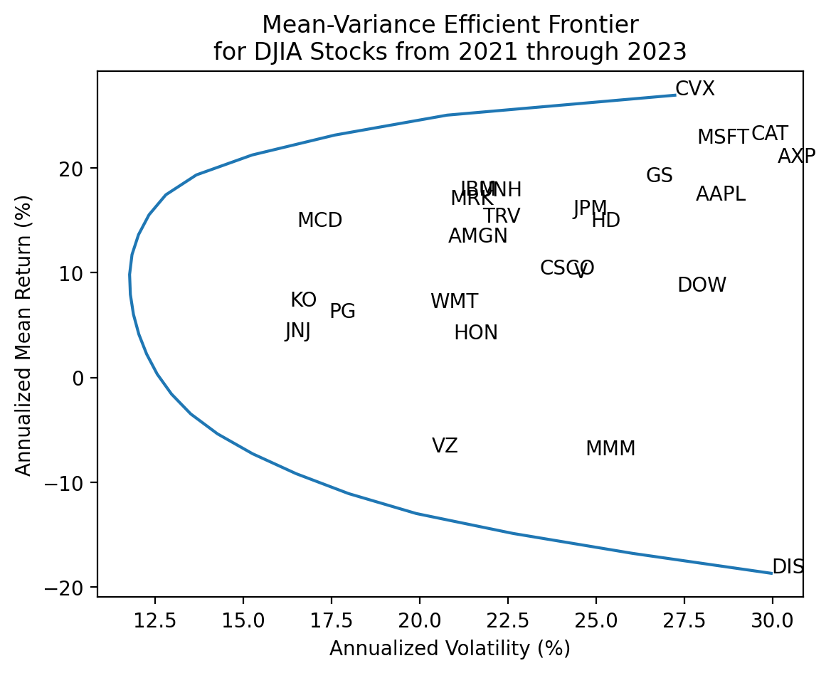
3.9 Find the maximum Sharpe Ratio portfolio with all available data for the current the DJIA stocks
res_sr_5 = sco.minimize(
    fun=calc_neg_sharpe,
    x0=djia.pipe(get_equal_weights),
    args=(djia.loc['2021':'2023'], ff['RF'], 252),
    bounds=((0, 1) for c in djia.columns),
    constraints=(
        {'type':'eq', 'fun': lambda x: x.sum() - 1}
    )
)

res_sr_5
message: Optimization terminated successfully
success: True
status: 0
fun: -1.2674934306134356
x: [ 0.000e+00 1.240e-02 ... 1.018e-15 0.000e+00]
nit: 9
jac: [ 1.679e-01 -1.458e-01 ... 1.165e+00 1.698e-01]
nfev: 282
njev: 9plt.barh(
y=djia.columns,
width=res_sr_5['x']
)
plt.ylabel('Ticker')
plt.xlabel('Portfolio Weight')
plt.title('Maximum Sharpe Ratio Portfolio Weights\n for DJIA Stocks from 2021 through 2023')
plt.show()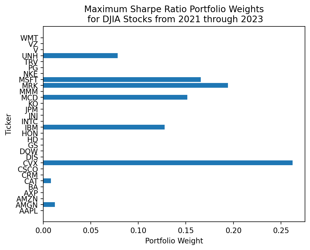
3.10 Compare the \(\frac{1}{n}\) and maximum Sharpe Ratio portfolios with all available data for the current DJIA stocks
Use all but the last 252 trading days to estimate the maximum Sharpe Ratio portfolio weights. Then use the last 252 trading days of data to compare the \(\frac{1}{n}\) maximum Sharpe Ratio portfolios.
res_sr_6 = sco.minimize(
    fun=calc_neg_sharpe,
    x0=djia.pipe(get_equal_weights),
    args=(djia.loc['2021':'2022'], ff['RF'], 252),
    bounds=((0, 1) for c in djia.columns),
    constraints=(
        {'type':'eq', 'fun': lambda x: x.sum() - 1}
    )
)

res_sr_6
message: Optimization terminated successfully
success: True
status: 0
fun: -1.8291517812610791
x: [ 2.365e-16 3.515e-16 ... 0.000e+00 9.216e-19]
nit: 7
jac: [ 8.874e-01 5.597e-02 ... 1.586e+00 5.228e-01]
nfev: 220
njev: 7plt.barh(
y=djia.columns,
width=res_sr_6['x'],
label='Maximum Sharpe Ratio Weights'
)
plt.axvline(1/30, color='red', label='Equal Weights')
plt.legend()
plt.ylabel('Ticker')
plt.xlabel('Portfolio Weight')
plt.title('Maximum Sharpe Ratio Portfolio Weights\n for DJIA Stocks from 2021 through 2023')
plt.show()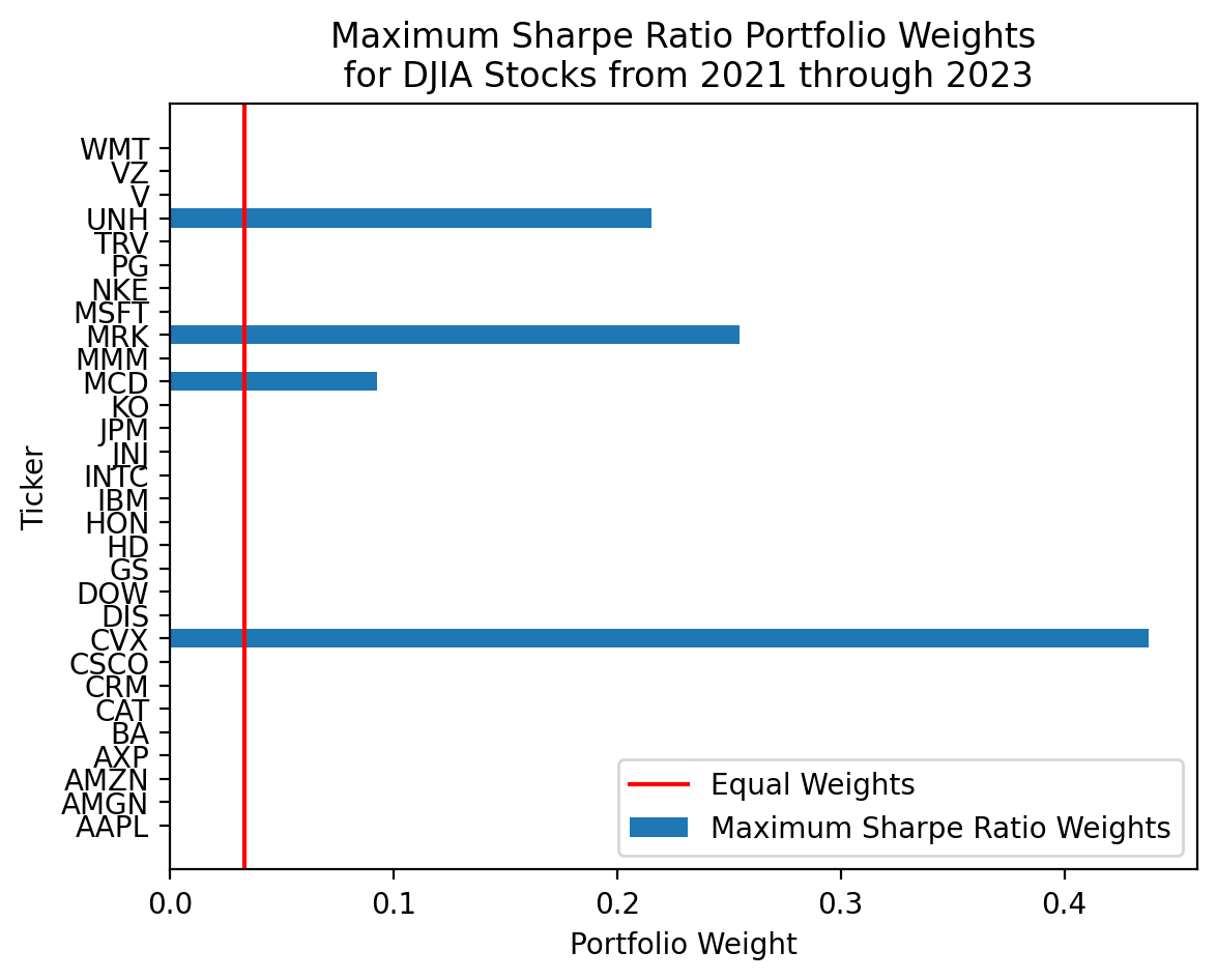
Here is the how max Sharpe portfolio does in 2023:
calc_sharpe(x=res_sr_6['x'], r=djia.loc['2023'], tgt=ff['RF'], ppy=252)-0.5146calc_sharpe(x=np.ones(djia.shape[1]) / djia.shape[1], r=djia.loc['2023'], tgt=ff['RF'], ppy=252)1.2388It is hard to beat the \(\frac{1}{n}\) portfolio because mean returns are hard to predict!