import matplotlib.pyplot as plt
import numpy as np
import pandas as pd
import yfinance as yfMcKinney Chapter 5 - Practice for Section 04
FINA 6333 for Spring 2024
1 Announcements
- No DataCamp this week, but I suggest you keep working on it
- Keep forming groups, and I will post our first project early next week
2 10-Minute Recap
%precision 4
pd.options.display.float_format = '{:.4f}'.format
%config InlineBackend.figure_format = 'retina'
pandas provides two data structures:
- Data frame is a 2-D, mixed data type structure, like a worksheet in an Excel workbook
- Series is a 1-D, one data type structure, like a column in a worksheet (or data frame)
np.random.seed(42)
df = pd.DataFrame(
    data=np.random.randn(3, 4), # 12 random numbers
    index=list('ABC'), # labels the rows for easy indexing and slicing
    columns=list('abcd') # labels the columns for easy indexing and slicing
)

df| a | b | c | d | |
|---|---|---|---|---|
| A | 0.4967 | -0.1383 | 0.6477 | 1.5230 |
| B | -0.2342 | -0.2341 | 1.5792 | 0.7674 |
| C | -0.4695 | 0.5426 | -0.4634 | -0.4657 |
How do we index or slice data frames?
- With integer locations and the
.iloc[]method - With row and column names and the
.loc[]method
Say we want the first two rows and first three columns.
df.iloc[:2, :3] # j,k slicing, as in NumPy| a | b | c | |
|---|---|---|---|
| A | 0.4967 | -0.1383 | 0.6477 |
| B | -0.2342 | -0.2341 | 1.5792 |
df.loc[['A', 'B'], ['a', 'b', 'c']]| a | b | c | |
|---|---|---|---|
| A | 0.4967 | -0.1383 | 0.6477 |
| B | -0.2342 | -0.2341 | 1.5792 |
Both left and right edges of named slices are included in pandas!
df.loc['A':'B', 'a':'c']| a | b | c | |
|---|---|---|---|
| A | 0.4967 | -0.1383 | 0.6477 |
| B | -0.2342 | -0.2341 | 1.5792 |
How do I add a column?
df['e'] = 5 # pandas broadcasts this 5 to all rows

df| a | b | c | d | e | |
|---|---|---|---|---|---|
| A | 0.4967 | -0.1383 | 0.6477 | 1.5230 | 5 |
| B | -0.2342 | -0.2341 | 1.5792 | 0.7674 | 5 |
| C | -0.4695 | 0.5426 | -0.4634 | -0.4657 | 5 |
A series is the other data structure.
ser = pd.Series(data=np.arange(2.), index=list('BC'))

ser
B 0.0000
C 1.0000
dtype: float64df['f'] = ser
df| a | b | c | d | e | f | |
|---|---|---|---|---|---|---|
| A | 0.4967 | -0.1383 | 0.6477 | 1.5230 | 5 | NaN |
| B | -0.2342 | -0.2341 | 1.5792 | 0.7674 | 5 | 0.0000 |
| C | -0.4695 | 0.5426 | -0.4634 | -0.4657 | 5 | 1.0000 |
3 Practice
tickers = 'AAPL IBM MSFT GOOG'
prices = yf.download(tickers=tickers)
[*********************100%%**********************] 4 of 4 completedreturns = (
prices['Adj Close'] # slices the adj close columns
.iloc[:-1] # drop last date with intraday price
.pct_change() # calculate returns
.dropna() # drop dates with incomplete returns data
)
returns| AAPL | GOOG | IBM | MSFT | |
|---|---|---|---|---|
| Date | ||||
| 2004-08-20 | 0.0029 | 0.0794 | 0.0042 | 0.0030 |
| 2004-08-23 | 0.0091 | 0.0101 | -0.0070 | 0.0044 |
| 2004-08-24 | 0.0280 | -0.0414 | 0.0007 | 0.0000 |
| 2004-08-25 | 0.0344 | 0.0108 | 0.0042 | 0.0114 |
| 2004-08-26 | 0.0487 | 0.0180 | -0.0045 | -0.0040 |
| ... | ... | ... | ... | ... |
| 2024-01-26 | -0.0090 | 0.0010 | -0.0158 | -0.0023 |
| 2024-01-29 | -0.0036 | 0.0068 | -0.0015 | 0.0143 |
| 2024-01-30 | -0.0192 | -0.0116 | 0.0039 | -0.0028 |
| 2024-01-31 | -0.0194 | -0.0735 | -0.0224 | -0.0269 |
| 2024-02-01 | 0.0133 | 0.0064 | 0.0176 | 0.0156 |
4896 rows × 4 columns
3.1 What are the mean daily returns for these four stocks?
returns.mean() # default is axis=0AAPL 0.0014
GOOG 0.0010
IBM 0.0004
MSFT 0.0008
dtype: float64If we use .mean(axis=1) on stock returns, we get the equallu-weighted portfolio returns on each day.
returns.mean(axis=1)Date
2004-08-20 0.0224
2004-08-23 0.0041
2004-08-24 -0.0032
2004-08-25 0.0152
2004-08-26 0.0146
...
2024-01-26 -0.0065
2024-01-29 0.0040
2024-01-30 -0.0074
2024-01-31 -0.0356
2024-02-01 0.0132
Length: 4896, dtype: float643.2 What are the standard deviations of daily returns for these four stocks?
pandas methods give us sample statistics, instead of population statistics in NumPy.
returns.std()AAPL 0.0206
GOOG 0.0194
IBM 0.0143
MSFT 0.0171
dtype: float643.3 What are the annualized means and standard deviations of daily returns for these four stocks?
We annualize mean returns by multiplying by \(T\) (\(T=252\) for daily returns, \(T=12\) for month returns, and so on). We annualize standard deviations by multiplying by \(\sqrt(T)\).
returns.mean().mul(252)AAPL 0.3625
GOOG 0.2552
IBM 0.0980
MSFT 0.2002
dtype: float64returns.std().mul(np.sqrt(252))AAPL 0.3276
GOOG 0.3074
IBM 0.2272
MSFT 0.2722
dtype: float643.4 Plot annualized means versus standard deviations of daily returns for these four stocks
means = returns.mean().mul(252 * 100)
vols = returns.std().mul(np.sqrt(252) * 100)

plt.scatter(
    x=vols,
    y=means
)

# add tickers to each point
for i in means.index: # loop over ticker index
    plt.text( # plots string s at coordinates x and y
        x=vols[i], # indexes volatility
        y=means[i], # indexes mean return
        s=i # ticker index
    )

plt.xlabel('Annualized Volatility of Daily Returns (%)')
plt.ylabel('Annualized Means of Daily Returns (%)')
plt.title('Returns versus Risk')
plt.show()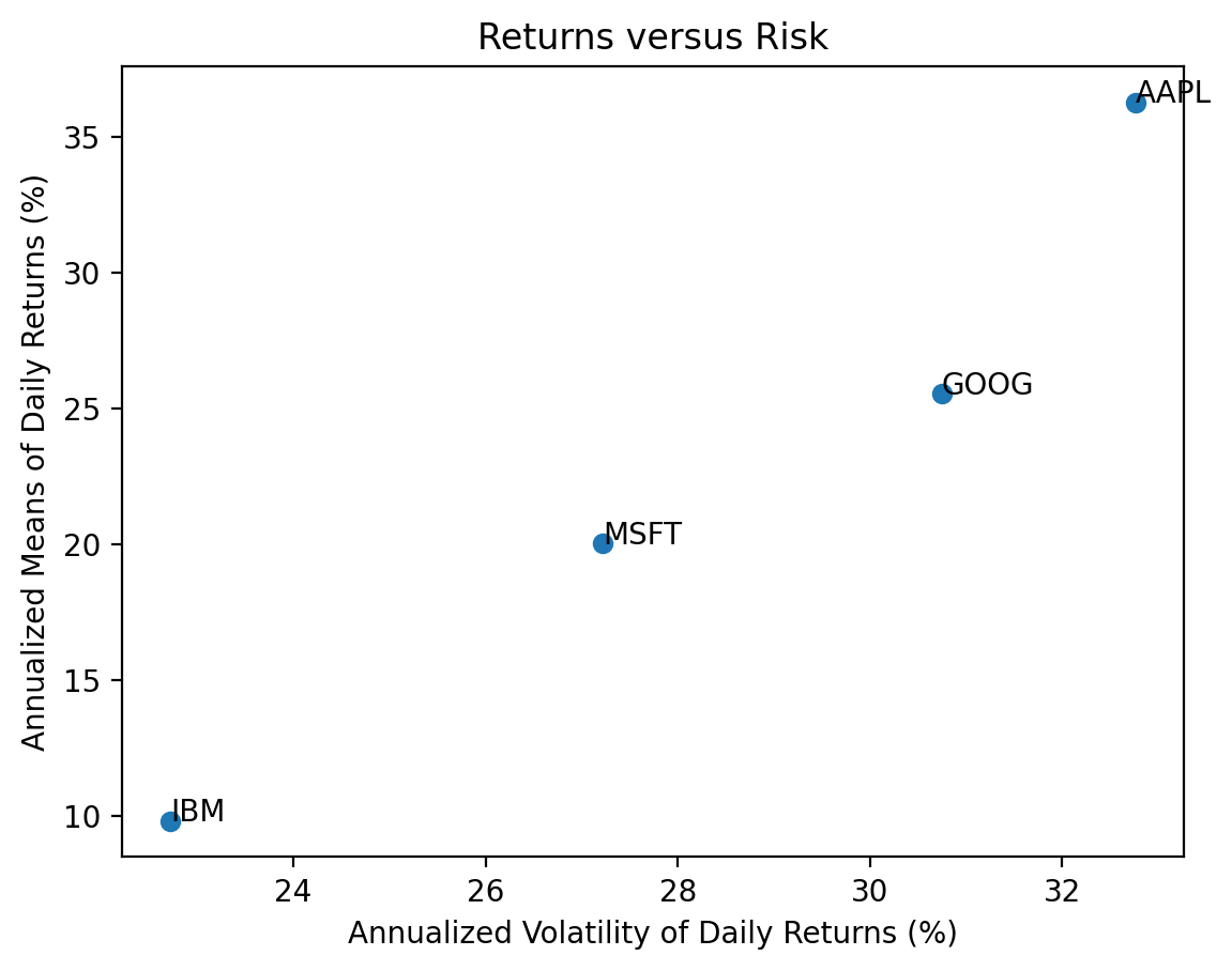
Use plt.scatter(), which expects arguments as x (standard deviations) then y (means).
3.5 Repeat the previous calculations and plot for the stocks in the Dow-Jones Industrial Index (DJIA)
We can find the current DJIA stocks on Wikipedia. We will need to download new data, into tickers2, prices2, and returns2.
url2 = 'https://en.wikipedia.org/wiki/Dow_Jones_Industrial_Average'
wiki2 = pd.read_html(url2)
tickers2 = wiki2[1]['Symbol'].to_list()
tickers2[:5]
['MMM', 'AXP', 'AMGN', 'AAPL', 'BA']prices2 = yf.download(tickers=tickers2)[*********************100%%**********************] 30 of 30 completedreturns2 = (
prices2['Adj Close']
.iloc[:-1]
.pct_change()
.dropna()
)
returns2| AAPL | AMGN | AXP | BA | CAT | CRM | CSCO | CVX | DIS | DOW | ... | MRK | MSFT | NKE | PG | TRV | UNH | V | VZ | WBA | WMT | |
|---|---|---|---|---|---|---|---|---|---|---|---|---|---|---|---|---|---|---|---|---|---|
| Date | |||||||||||||||||||||
| 2019-03-21 | 0.0368 | 0.0040 | 0.0095 | -0.0092 | 0.0079 | 0.0210 | 0.0128 | 0.0094 | -0.0121 | -0.0165 | ... | 0.0106 | 0.0230 | 0.0152 | 0.0076 | 0.0231 | 0.0061 | 0.0133 | 0.0108 | 0.0129 | 0.0043 |
| 2019-03-22 | -0.0207 | -0.0270 | -0.0211 | -0.0283 | -0.0320 | -0.0326 | -0.0222 | -0.0220 | -0.0040 | -0.0078 | ... | -0.0080 | -0.0264 | -0.0661 | -0.0081 | 0.0039 | -0.0196 | -0.0175 | 0.0252 | -0.0187 | -0.0079 |
| 2019-03-25 | -0.0121 | -0.0006 | -0.0038 | 0.0229 | 0.0124 | -0.0038 | -0.0002 | -0.0016 | -0.0041 | 0.0113 | ... | 0.0007 | 0.0052 | 0.0017 | 0.0030 | 0.0004 | -0.0009 | -0.0003 | 0.0054 | -0.0115 | -0.0011 |
| 2019-03-26 | -0.0103 | 0.0090 | 0.0042 | -0.0002 | 0.0035 | -0.0092 | 0.0095 | 0.0101 | 0.0218 | -0.0061 | ... | 0.0069 | 0.0021 | 0.0128 | 0.0104 | 0.0002 | -0.0141 | 0.0148 | 0.0092 | 0.0037 | 0.0015 |
| 2019-03-27 | 0.0090 | -0.0104 | -0.0047 | 0.0103 | -0.0049 | -0.0269 | -0.0017 | -0.0108 | 0.0013 | 0.0256 | ... | -0.0076 | -0.0097 | -0.0035 | -0.0012 | 0.0101 | -0.0069 | -0.0070 | 0.0041 | 0.0050 | -0.0113 |
| ... | ... | ... | ... | ... | ... | ... | ... | ... | ... | ... | ... | ... | ... | ... | ... | ... | ... | ... | ... | ... | ... |
| 2024-01-26 | -0.0090 | 0.0049 | 0.0710 | 0.0178 | -0.0045 | 0.0033 | -0.0036 | 0.0038 | 0.0053 | -0.0160 | ... | 0.0057 | -0.0023 | 0.0196 | 0.0033 | -0.0004 | 0.0199 | -0.0171 | 0.0026 | -0.0113 | 0.0088 |
| 2024-01-29 | -0.0036 | 0.0054 | -0.0028 | -0.0014 | 0.0128 | 0.0283 | 0.0029 | -0.0004 | 0.0223 | 0.0002 | ... | 0.0038 | 0.0143 | 0.0110 | 0.0001 | -0.0015 | 0.0027 | 0.0213 | -0.0083 | -0.0057 | 0.0047 |
| 2024-01-30 | -0.0192 | 0.0037 | 0.0164 | -0.0231 | 0.0050 | -0.0005 | -0.0010 | 0.0070 | -0.0056 | 0.0074 | ... | 0.0031 | -0.0028 | 0.0029 | 0.0085 | 0.0115 | -0.0018 | 0.0128 | 0.0100 | 0.0018 | 0.0033 |
| 2024-01-31 | -0.0194 | -0.0011 | -0.0167 | 0.0529 | -0.0146 | -0.0231 | -0.0394 | -0.0179 | -0.0092 | -0.0160 | ... | -0.0072 | -0.0269 | -0.0254 | -0.0022 | -0.0102 | 0.0161 | -0.0140 | -0.0028 | -0.0083 | -0.0021 |
| 2024-02-01 | 0.0133 | 0.0328 | 0.0124 | -0.0058 | 0.0246 | 0.0096 | 0.0000 | 0.0031 | 0.0105 | -0.0011 | ... | 0.0464 | 0.0156 | 0.0023 | 0.0130 | 0.0031 | -0.0090 | 0.0139 | 0.0033 | 0.0301 | 0.0185 |
1226 rows × 30 columns
means = returns2.mean().mul(252 * 100)
vols = returns2.std().mul(np.sqrt(252) * 100)

plt.scatter(
    x=vols,
    y=means
)

# add tickers to each point
for i in means.index: # loop over ticker index
    plt.text( # plots string s at coordinates x and y
        x=vols[i], # indexes volatility
        y=means[i], # indexes mean return
        s=i # ticker index
    )

plt.xlabel('Annualized Volatility of Daily Returns (%)')
plt.ylabel('Annualized Means of Daily Returns (%)')
plt.title('Returns versus Risk')
plt.show()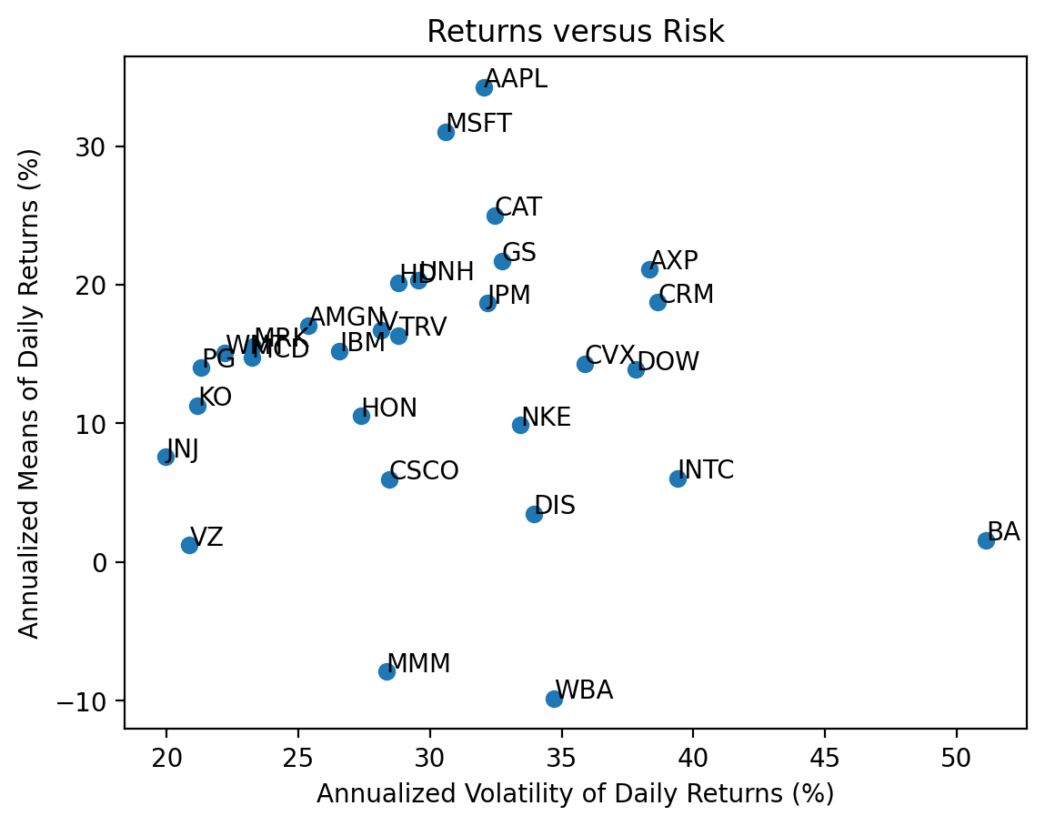
3.6 Calculate total returns for the stocks in the DJIA
We can use the .prod() method to compound returns as \(1 + R_T = \prod_{t=1}^T (1 + R_t)\). Technically, we should write \(R_T\) as \(R_{0,T}\), but we typically omit the subscript \(0\).
total_returns2 = returns2.add(1).prod().sub(1)
total_returns2.iloc[:5]
AAPL 3.1210
AMGN 0.9635
AXP 0.9687
BA -0.4289
CAT 1.6083
dtype: float643.7 Plot the distribution of total returns for the stocks in the DJIA
We can plot a histogram, using either the plt.hist() function or the .plot(kind='hist') method.
start_date = returns2.index.min()
stop_date = returns2.index.max()

(
    returns2
    .add(1)
    .prod()
    .sub(1)
    .mul(100)
    .plot(kind='hist', bins=20)
)
plt.xlabel('Total Return (%)')
plt.title(f'Distribution of Total Returns for DJIA Stocks\n from {start_date:%B %Y} to {stop_date:%B %Y}')
plt.show()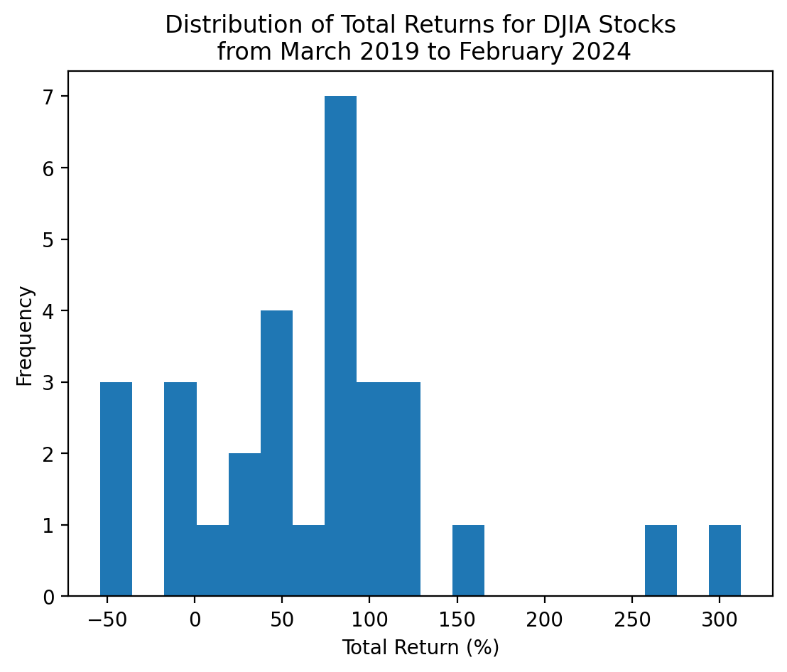
With only 30 stocks, we can visualize and interpret each stock separately!
start_date = returns2.index.min()
stop_date = returns2.index.max()

(
    returns2
    .add(1)
    .prod()
    .sub(1)
    .mul(100)
    .sort_values()
    .plot(kind='barh', grid=True)
)
plt.xlabel('Total Return (%)')
plt.title(f'Total Returns for DJIA Stocks\n from {start_date:%B %Y} to {stop_date:%B %Y}')
plt.show()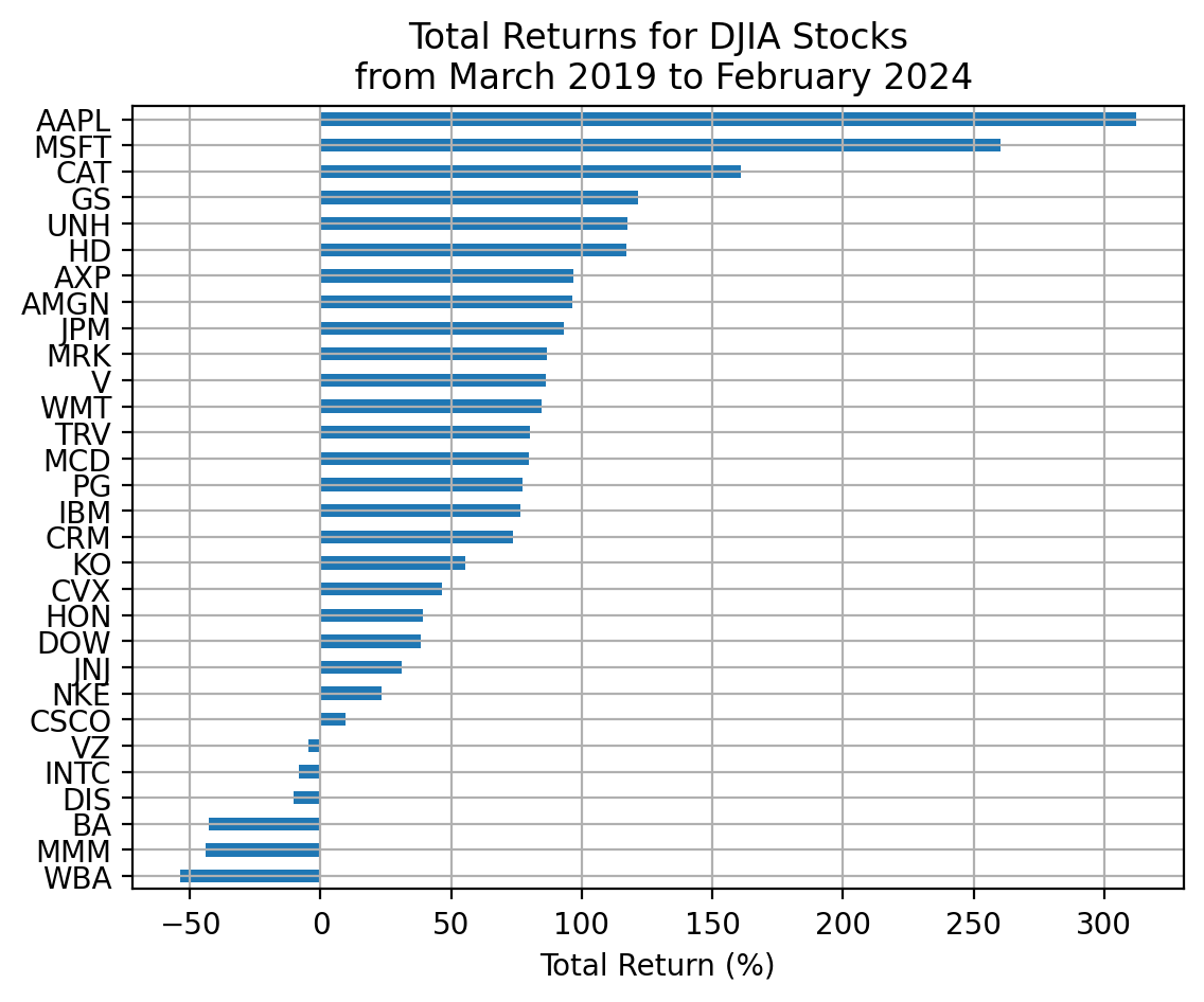
3.8 Which stocks have the minimum and maximum total returns?
If we want the values, the .min() and .max() methods are the way to go!
total_returns2.min()-0.5384total_returns2.max()3.1210The .min() and .max() methods give the values but not the tickers (or index). We use the .idxmin() and .idxmax() to get the tickers (or index).
total_returns2.idxmin()'WBA'total_returns2.idxmax()'AAPL'Here is what I would use!
total_returns2.sort_values().iloc[[0, -1]]WBA -0.5384
AAPL 3.1210
dtype: float64Not the exactly right tool here, but the .nsmallest()' and.nlargest()` methods are really useful!
total_returns2.nsmallest(3)WBA -0.5384
MMM -0.4408
BA -0.4289
dtype: float64total_returns2.nlargest(3)AAPL 3.1210
MSFT 2.6028
CAT 1.6083
dtype: float643.9 Plot the cumulative returns for the stocks in the DJIA
We can use the cumulative product method .cumprod() to calculate the right hand side of the formula above.
start_date = returns2.index.min()
stop_date = returns2.index.max()

(
    returns2
    .add(1)
    .cumprod()
    .sub(1)
    .mul(100)
    .plot(legend=False)
)
plt.ylabel('Cumulative Return (%)')
plt.title(f'Cumulative Returns on DJIA Stocks\n from {start_date:%B %Y} to {stop_date:%B %Y}')
plt.show()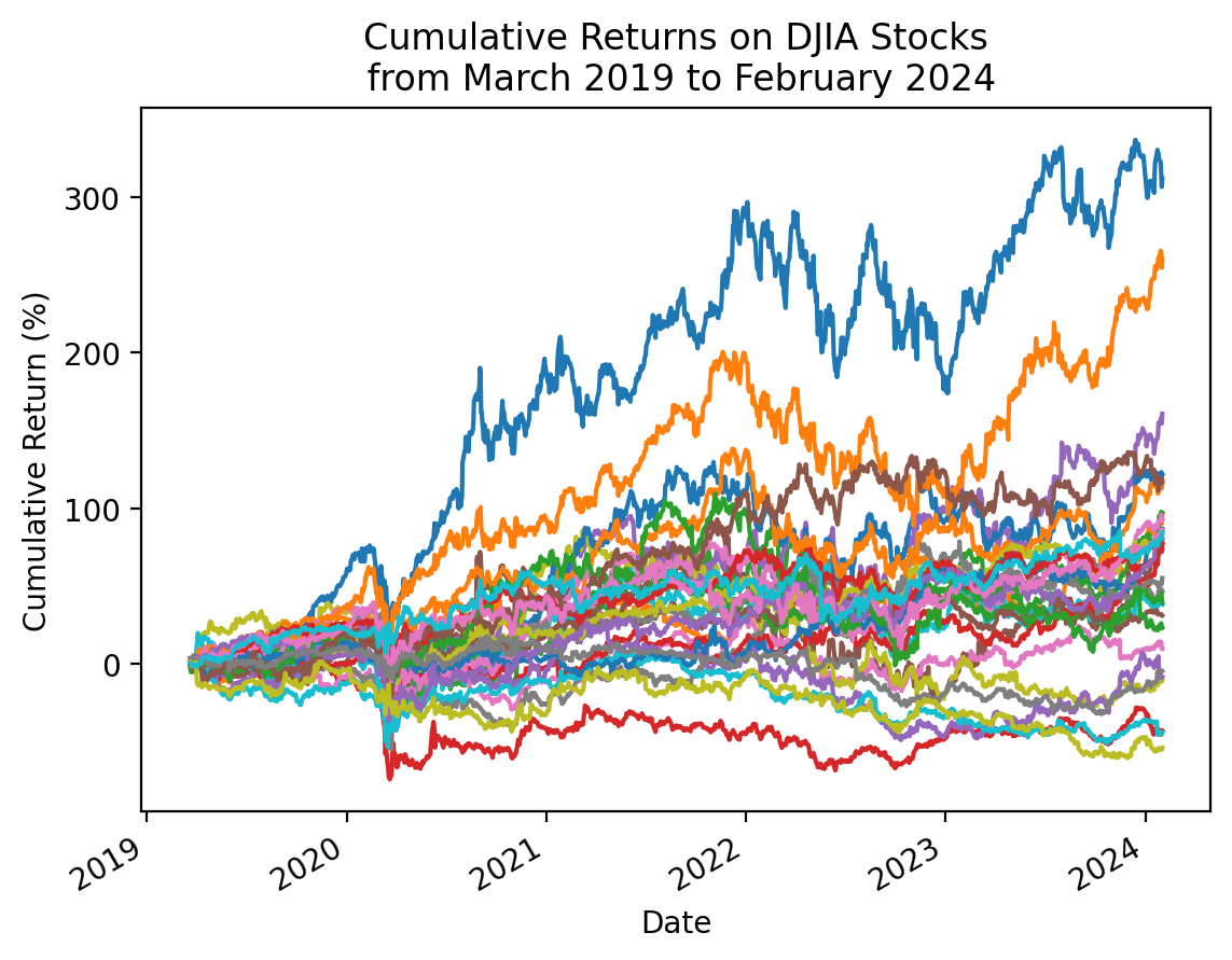
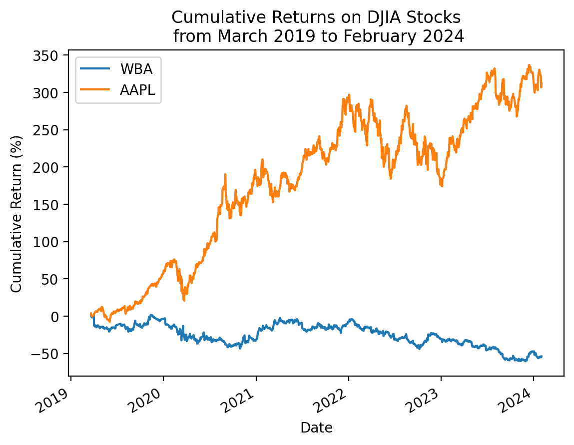
3.10 Repeat the plot above with only the minimum and maximum total returns
total_returns2.sort_values().iloc[[0, -1]].indexIndex(['WBA', 'AAPL'], dtype='object')start_date = returns2.index.min()
stop_date = returns2.index.max()
(
returns2[total_returns2.sort_values().iloc[[0, -1]].index]
.add(1)
.cumprod()
.sub(1)
.mul(100)
.plot()
)
plt.ylabel('Cumulative Return (%)')
plt.title(f'Cumulative Returns on DJIA Stocks\n from {start_date:%B %Y} to {stop_date:%B %Y}')
plt.show()