import matplotlib.pyplot as plt
import numpy as np
import pandas as pd
import yfinance as yfMcKinney Chapter 5 - Practice for Section 03
FINA 6333 for Spring 2024
1 Announcements
- No DataCamp this week, but I suggest you keep working on it
- Keep forming groups, and I will post our first project early next week
2 10-Minute Recap
%precision 4
pd.options.display.float_format = '{:.4f}'.format
%config InlineBackend.figure_format = 'retina'
pandas provides two very useful data structures:
- Data frames are like a worksheet in an Excel workbook (2-D, mixed data type)
- Series are like a column in a worksheet in an Excel workbook (1-D, one data type)
np.random.seed(42)
df = pd.DataFrame(
    data=np.random.randn(4, 4),
    index=list('ABCD'),
    columns=list('abcd')
)

df| a | b | c | d | |
|---|---|---|---|---|
| A | 0.4967 | -0.1383 | 0.6477 | 1.5230 |
| B | -0.2342 | -0.2341 | 1.5792 | 0.7674 |
| C | -0.4695 | 0.5426 | -0.4634 | -0.4657 |
| D | 0.2420 | -1.9133 | -1.7249 | -0.5623 |
How can we slice the first two rows and three columns? We can slice data frames two ways:
- Using integer locations and the
.iloc[]method - Using row and column names with the
.loc[]method
df.iloc[:2, :3] # slice with j,k notation, like NumPy| a | b | c | |
|---|---|---|---|
| A | 0.4967 | -0.1383 | 0.6477 |
| B | -0.2342 | -0.2341 | 1.5792 |
When we slice by names or labels, we get both left and right edges included!
df.loc['A':'B', 'a':'c']| a | b | c | |
|---|---|---|---|
| A | 0.4967 | -0.1383 | 0.6477 |
| B | -0.2342 | -0.2341 | 1.5792 |
We can easily add columns!
df['e'] = 5 # broadcasts to every row in df

df| a | b | c | d | e | |
|---|---|---|---|---|---|
| A | 0.4967 | -0.1383 | 0.6477 | 1.5230 | 5 |
| B | -0.2342 | -0.2341 | 1.5792 | 0.7674 | 5 |
| C | -0.4695 | 0.5426 | -0.4634 | -0.4657 | 5 |
| D | 0.2420 | -1.9133 | -1.7249 | -0.5623 | 5 |
df['e'] = np.random.randn(4)

df| a | b | c | d | e | |
|---|---|---|---|---|---|
| A | 0.4967 | -0.1383 | 0.6477 | 1.5230 | -1.0128 |
| B | -0.2342 | -0.2341 | 1.5792 | 0.7674 | 0.3142 |
| C | -0.4695 | 0.5426 | -0.4634 | -0.4657 | -0.9080 |
| D | 0.2420 | -1.9133 | -1.7249 | -0.5623 | -1.4123 |
A series is the other, 1-D data structure in pandas!
ser = pd.Series(data=np.arange(2.), index=['C', 'D']) # the . in np.arange() makes the array floats

ser
C 0.0000
D 1.0000
dtype: float64df['f'] = ser
df| a | b | c | d | e | f | |
|---|---|---|---|---|---|---|
| A | 0.4967 | -0.1383 | 0.6477 | 1.5230 | -1.0128 | NaN |
| B | -0.2342 | -0.2341 | 1.5792 | 0.7674 | 0.3142 | NaN |
| C | -0.4695 | 0.5426 | -0.4634 | -0.4657 | -0.9080 | 0.0000 |
| D | 0.2420 | -1.9133 | -1.7249 | -0.5623 | -1.4123 | 1.0000 |
3 Practice
tickers = 'AAPL IBM MSFT GOOG'
prices = yf.download(tickers=tickers)
[*********************100%%**********************] 4 of 4 completedreturns = (
prices['Adj Close'] # slice adj close column
.iloc[:-1] # drop last row with intra day prices, which are sometimes missing
.pct_change() # calculate returns
.dropna() # drop leading rows with at least one missing value
)
returns| AAPL | GOOG | IBM | MSFT | |
|---|---|---|---|---|
| Date | ||||
| 2004-08-20 | 0.0029 | 0.0794 | 0.0042 | 0.0030 |
| 2004-08-23 | 0.0091 | 0.0101 | -0.0070 | 0.0044 |
| 2004-08-24 | 0.0280 | -0.0414 | 0.0007 | 0.0000 |
| 2004-08-25 | 0.0344 | 0.0108 | 0.0042 | 0.0114 |
| 2004-08-26 | 0.0487 | 0.0180 | -0.0045 | -0.0040 |
| ... | ... | ... | ... | ... |
| 2024-01-26 | -0.0090 | 0.0010 | -0.0158 | -0.0023 |
| 2024-01-29 | -0.0036 | 0.0068 | -0.0015 | 0.0143 |
| 2024-01-30 | -0.0192 | -0.0116 | 0.0039 | -0.0028 |
| 2024-01-31 | -0.0194 | -0.0735 | -0.0224 | -0.0269 |
| 2024-02-01 | 0.0133 | 0.0064 | 0.0176 | 0.0156 |
4896 rows × 4 columns
3.1 What are the mean daily returns for these four stocks?
returns.mean() # default axis=0 takes the mean of each columnAAPL 0.0014
GOOG 0.0010
IBM 0.0004
MSFT 0.0008
dtype: float64If we pass axis=1, we get the mean return on each day. We can this an “equally-weighted portfolio return.” \[r_{p,t} = \sum_{i=0}^4 \frac{1}{4} r_{i, t}\]
returns.mean(axis=1)Date
2004-08-20 0.0224
2004-08-23 0.0041
2004-08-24 -0.0032
2004-08-25 0.0152
2004-08-26 0.0146
...
2024-01-26 -0.0065
2024-01-29 0.0040
2024-01-30 -0.0074
2024-01-31 -0.0356
2024-02-01 0.0132
Length: 4896, dtype: float643.2 What are the standard deviations of daily returns for these four stocks?
pandas calcualates sample statistics by default.
returns.std()AAPL 0.0206
GOOG 0.0194
IBM 0.0143
MSFT 0.0171
dtype: float643.3 What are the annualized means and standard deviations of daily returns for these four stocks?
We annualize mean returns by multiplying by \(T\) (\(T=252\) for daily returns, \(T=12\) for month returns, and so on). We annualize standard deviations by multiplying by \(\sqrt(T)\).
returns.mean().mul(252)AAPL 0.3625
GOOG 0.2552
IBM 0.0980
MSFT 0.2002
dtype: float64returns.std().mul(np.sqrt(252))AAPL 0.3276
GOOG 0.3074
IBM 0.2272
MSFT 0.2722
dtype: float643.4 Plot annualized means versus standard deviations of daily returns for these four stocks
Use plt.scatter(), which expects arguments as x (standard deviations) then y (means).
vols = returns.std().mul(np.sqrt(252) * 100)
means = returns.mean().mul(252 * 100)

plt.scatter(
    x=vols,
    y=means
)

# add tickers to each point
for i in means.index: # loop over ticker index
    plt.text( # plots string s at coordinates x and y
        x=vols[i], # indexes volatility
        y=means[i], # indexes mean return
        s=i # ticker index
    )

plt.xlabel('Annualized Volatility of Daily Returns (%)')
plt.ylabel('Annualized Mean of Daily Returns (%)')

plt.title('Returns versus Risk')
plt.show()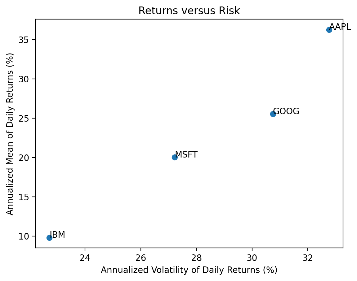
3.5 Repeat the previous calculations and plot for the stocks in the Dow-Jones Industrial Index (DJIA)
We can find the current DJIA stocks on Wikipedia. We will need to download new data, into tickers2, prices2, and returns2.
url2 = 'https://en.wikipedia.org/wiki/Dow_Jones_Industrial_Average'
wiki2 = pd.read_html(io=url2)
tickers2 = wiki2[1]['Symbol'].to_list()
tickers2[:5]
['MMM', 'AXP', 'AMGN', 'AAPL', 'BA']prices2 = yf.download(tickers=tickers2)[*********************100%%**********************] 30 of 30 completedreturns2 = (
prices2['Adj Close'] # slide adj close for all stocks
.iloc[:-1] # drop last day of adj close, which are intraday values before 4 PM
.pct_change() # calculate returns
.dropna() # drop any dates with incomplete data
)
returns2| AAPL | AMGN | AXP | BA | CAT | CRM | CSCO | CVX | DIS | DOW | ... | MRK | MSFT | NKE | PG | TRV | UNH | V | VZ | WBA | WMT | |
|---|---|---|---|---|---|---|---|---|---|---|---|---|---|---|---|---|---|---|---|---|---|
| Date | |||||||||||||||||||||
| 2019-03-21 | 0.0368 | 0.0040 | 0.0095 | -0.0092 | 0.0079 | 0.0210 | 0.0128 | 0.0094 | -0.0121 | -0.0165 | ... | 0.0106 | 0.0230 | 0.0152 | 0.0076 | 0.0231 | 0.0061 | 0.0133 | 0.0108 | 0.0129 | 0.0043 |
| 2019-03-22 | -0.0207 | -0.0270 | -0.0211 | -0.0283 | -0.0320 | -0.0326 | -0.0222 | -0.0220 | -0.0040 | -0.0078 | ... | -0.0080 | -0.0264 | -0.0661 | -0.0081 | 0.0039 | -0.0196 | -0.0175 | 0.0252 | -0.0187 | -0.0079 |
| 2019-03-25 | -0.0121 | -0.0006 | -0.0038 | 0.0229 | 0.0124 | -0.0038 | -0.0002 | -0.0016 | -0.0041 | 0.0113 | ... | 0.0007 | 0.0052 | 0.0017 | 0.0030 | 0.0004 | -0.0009 | -0.0003 | 0.0054 | -0.0115 | -0.0011 |
| 2019-03-26 | -0.0103 | 0.0090 | 0.0042 | -0.0002 | 0.0035 | -0.0092 | 0.0095 | 0.0101 | 0.0218 | -0.0061 | ... | 0.0069 | 0.0021 | 0.0128 | 0.0104 | 0.0002 | -0.0141 | 0.0148 | 0.0092 | 0.0037 | 0.0015 |
| 2019-03-27 | 0.0090 | -0.0104 | -0.0047 | 0.0103 | -0.0049 | -0.0269 | -0.0017 | -0.0108 | 0.0013 | 0.0256 | ... | -0.0076 | -0.0097 | -0.0035 | -0.0012 | 0.0102 | -0.0069 | -0.0070 | 0.0041 | 0.0050 | -0.0113 |
| ... | ... | ... | ... | ... | ... | ... | ... | ... | ... | ... | ... | ... | ... | ... | ... | ... | ... | ... | ... | ... | ... |
| 2024-01-26 | -0.0090 | 0.0049 | 0.0710 | 0.0178 | -0.0045 | 0.0033 | -0.0036 | 0.0038 | 0.0053 | -0.0160 | ... | 0.0057 | -0.0023 | 0.0196 | 0.0033 | -0.0004 | 0.0199 | -0.0171 | 0.0026 | -0.0113 | 0.0088 |
| 2024-01-29 | -0.0036 | 0.0054 | -0.0028 | -0.0014 | 0.0128 | 0.0283 | 0.0029 | -0.0004 | 0.0223 | 0.0002 | ... | 0.0038 | 0.0143 | 0.0110 | 0.0001 | -0.0015 | 0.0027 | 0.0213 | -0.0083 | -0.0057 | 0.0047 |
| 2024-01-30 | -0.0192 | 0.0037 | 0.0164 | -0.0231 | 0.0050 | -0.0005 | -0.0010 | 0.0070 | -0.0056 | 0.0074 | ... | 0.0031 | -0.0028 | 0.0029 | 0.0085 | 0.0115 | -0.0018 | 0.0128 | 0.0100 | 0.0018 | 0.0033 |
| 2024-01-31 | -0.0194 | -0.0011 | -0.0167 | 0.0529 | -0.0146 | -0.0231 | -0.0394 | -0.0179 | -0.0092 | -0.0160 | ... | -0.0072 | -0.0269 | -0.0254 | -0.0022 | -0.0102 | 0.0161 | -0.0140 | -0.0028 | -0.0083 | -0.0021 |
| 2024-02-01 | 0.0133 | 0.0328 | 0.0124 | -0.0058 | 0.0246 | 0.0096 | 0.0000 | 0.0031 | 0.0105 | -0.0011 | ... | 0.0464 | 0.0156 | 0.0023 | 0.0130 | 0.0031 | -0.0090 | 0.0139 | 0.0033 | 0.0301 | 0.0185 |
1226 rows × 30 columns
vols = returns2.std().mul(np.sqrt(252) * 100)
means = returns2.mean().mul(252 * 100)

plt.scatter(
    x=vols,
    y=means
)

# add tickers to each point
for i in means.index: # loop over ticker index
    plt.text( # plots string s at coordinates x and y
        x=vols[i], # indexes volatility
        y=means[i], # indexes mean return
        s=i # ticker index
    )

plt.xlabel('Annualized Volatility of Daily Returns (%)')
plt.ylabel('Annualized Mean of Daily Returns (%)')

plt.title('Returns versus Risk')
plt.show()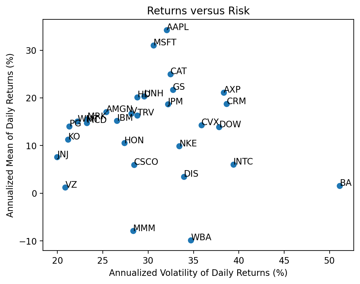
3.6 Calculate total returns for the stocks in the DJIA
We can use the .prod() method to compound returns as \(1 + R_T = \prod_{t=1}^T (1 + R_t)\). Technically, we should write \(R_T\) as \(R_{0,T}\), but we typically omit the subscript \(0\).
total_returns2 = returns2.add(1).prod().sub(1)

total_returns2.iloc[:5]
AAPL 3.1210
AMGN 0.9635
AXP 0.9687
BA -0.4289
CAT 1.6083
dtype: float64np.allclose(((returns2 + 1).prod() - 1), total_returns2)True3.7 Plot the distribution of total returns for the stocks in the DJIA
We can plot a histogram, using either the plt.hist() function or the .plot(kind='hist') method.
start_date = returns2.index.min()
stop_date = returns2.index.max()

(
    returns2
    .add(1)
    .prod()
    .sub(1)
    .mul(100)
    .plot(kind='hist', bins=20)
)
plt.xlabel('Total Return (%)')
plt.title(f'Distribution of Total Returns for DJIA Stocks\n from {start_date:%B %Y} to {stop_date:%B %Y}')
plt.show()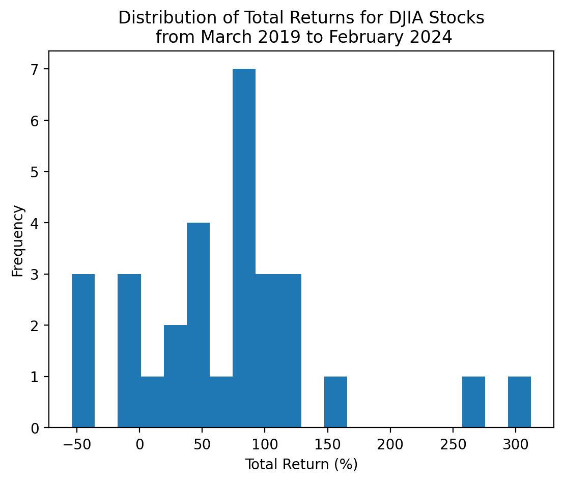
With only 30 stocks, we can visualize and interpret each stock separately!
start_date = returns2.index.min()
stop_date = returns2.index.max()

(
    returns2
    .add(1)
    .prod()
    .sub(1)
    .mul(100)
    .sort_values()
    .plot(kind='barh', grid=True)
)
plt.xlabel('Total Return (%)')
plt.title(f'Total Returns for DJIA Stocks\n from {start_date:%B %Y} to {stop_date:%B %Y}')
plt.show()
3.8 Which stocks have the minimum and maximum total returns?
If we want the values, the .min() and .max() methods are the way to go!
total_returns2.min()-0.5384total_returns2.max()3.1210The .min() and .max() methods give the values but not the tickers (or index). We use the .idxmin() and .idxmax() to get the tickers (or index).
total_returns2.idxmin()'WBA'total_returns2.idxmax()'AAPL'Here is what I would use!
total_returns2.sort_values().iloc[[0, -1]]WBA -0.5384
AAPL 3.1210
dtype: float64Not the exactly right tool here, but the .nsmallest()' and.nlargest()` methods are really useful!
total_returns2.nsmallest(3)WBA -0.5384
MMM -0.4408
BA -0.4289
dtype: float64total_returns2.nlargest(3)AAPL 3.1210
MSFT 2.6028
CAT 1.6083
dtype: float643.9 Plot the cumulative returns for the stocks in the DJIA
We can use the cumulative product method .cumprod() to calculate the right hand side of the formula above.
start_date = returns2.index.min()
stop_date = returns2.index.max()

(
    returns2
    .add(1)
    .cumprod()
    .sub(1)
    .mul(100)
    .plot(legend=False)
)
plt.xlabel('Cumulative Return (%)')
plt.title(f'Cumulative Returns for DJIA Stocks\n from {start_date:%B %Y} to {stop_date:%B %Y}')
plt.show()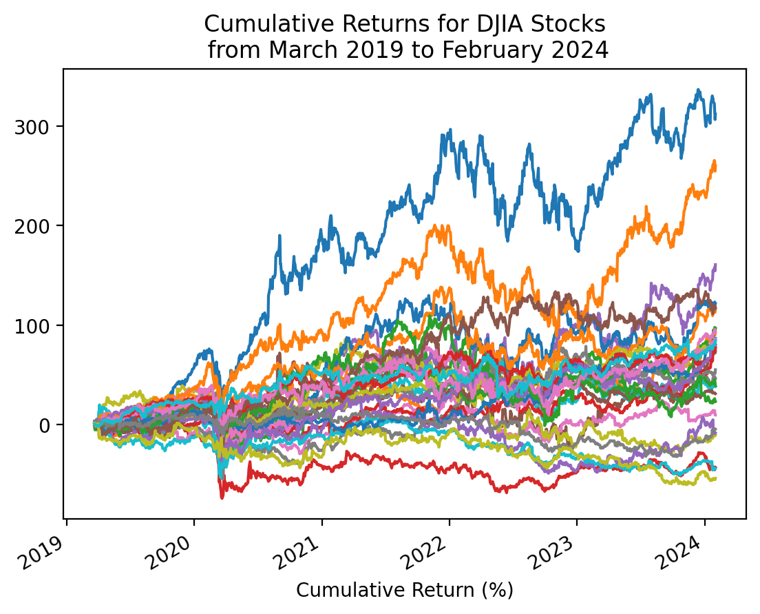
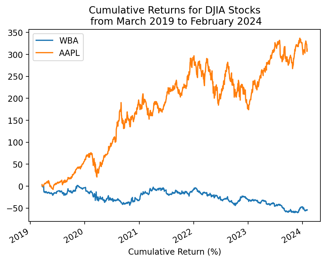
3.10 Repeat the plot above with only the minimum and maximum total returns
total_returns2.sort_values().iloc[[0, -1]].indexIndex(['WBA', 'AAPL'], dtype='object')start_date = returns2.index.min()
stop_date = returns2.index.max()
(
returns2[total_returns2.sort_values().iloc[[0, -1]].index]
.add(1)
.cumprod()
.sub(1)
.mul(100)
.plot()
)
plt.xlabel('Cumulative Return (%)')
plt.title(f'Cumulative Returns for DJIA Stocks\n from {start_date:%B %Y} to {stop_date:%B %Y}')
plt.show()