import matplotlib.pyplot as plt
import numpy as np
import pandas as pdHerron Topic 1 - Web Data, Log and Simple Returns, and Portfolio Math
FINA 6333 for Spring 2024
This notebook covers three topics:
- How to download web data with the yfinance and pandas-datareader packages
- How to calculate log and simple returns
- How to calculate portfolio returns
%precision 4
pd.options.display.float_format = '{:.4f}'.format
%config InlineBackend.figure_format = 'retina'
1 Web Data
We will typically use the yfinance and pandas-datarader packages to download data from the web. If you followed my instructions to install Miniconda on your computer, you have already installed these packages.
1.1 The yfinance Package
The yfinance package provides “a reliable, threaded, and Pythonic way to download historical market data from Yahoo! finance.” Other packages provide similar functionality, but yfinance is best.
import yfinance as yfWe can download data for the MATANA stocks (Microsoft, Alphabet, Tesla, Amazon, Nvidia, and Apple). We can pass tickers as either a space-delimited string or a list of strings.
df = yf.download(tickers='MSFT GOOG TSLA AMZN NVDA AAPL')
df
[*********************100%%**********************] 6 of 6 completed| Adj Close | Close | ... | Open | Volume | |||||||||||||||||
|---|---|---|---|---|---|---|---|---|---|---|---|---|---|---|---|---|---|---|---|---|---|
| AAPL | AMZN | GOOG | MSFT | NVDA | TSLA | AAPL | AMZN | GOOG | MSFT | ... | GOOG | MSFT | NVDA | TSLA | AAPL | AMZN | GOOG | MSFT | NVDA | TSLA | |
| Date | |||||||||||||||||||||
| 1980-12-12 | 0.0993 | NaN | NaN | NaN | NaN | NaN | 0.1283 | NaN | NaN | NaN | ... | NaN | NaN | NaN | NaN | 469033600 | NaN | NaN | NaN | NaN | NaN |
| 1980-12-15 | 0.0941 | NaN | NaN | NaN | NaN | NaN | 0.1217 | NaN | NaN | NaN | ... | NaN | NaN | NaN | NaN | 175884800 | NaN | NaN | NaN | NaN | NaN |
| 1980-12-16 | 0.0872 | NaN | NaN | NaN | NaN | NaN | 0.1127 | NaN | NaN | NaN | ... | NaN | NaN | NaN | NaN | 105728000 | NaN | NaN | NaN | NaN | NaN |
| 1980-12-17 | 0.0894 | NaN | NaN | NaN | NaN | NaN | 0.1155 | NaN | NaN | NaN | ... | NaN | NaN | NaN | NaN | 86441600 | NaN | NaN | NaN | NaN | NaN |
| 1980-12-18 | 0.0920 | NaN | NaN | NaN | NaN | NaN | 0.1189 | NaN | NaN | NaN | ... | NaN | NaN | NaN | NaN | 73449600 | NaN | NaN | NaN | NaN | NaN |
| ... | ... | ... | ... | ... | ... | ... | ... | ... | ... | ... | ... | ... | ... | ... | ... | ... | ... | ... | ... | ... | ... |
| 2024-01-26 | 192.4200 | 159.1200 | 153.7900 | 403.9300 | 610.3100 | 183.2500 | 192.4200 | 159.1200 | 153.7900 | 403.9300 | ... | 152.8700 | 404.3700 | 609.6000 | 185.5000 | 44553400 | 51001100.0000 | 19483600.0000 | 17786700.0000 | 38983800.0000 | 107063400.0000 |
| 2024-01-29 | 191.7300 | 161.2600 | 154.8400 | 409.7200 | 624.6500 | 190.9300 | 191.7300 | 161.2600 | 154.8400 | 409.7200 | ... | 153.6400 | 406.0600 | 612.3200 | 185.6300 | 47145600 | 45270400.0000 | 20909300.0000 | 24510200.0000 | 34873300.0000 | 125013100.0000 |
| 2024-01-30 | 188.0400 | 159.0000 | 153.0500 | 408.5900 | 627.7400 | 191.5900 | 188.0400 | 159.0000 | 153.0500 | 408.5900 | ... | 154.0100 | 412.2600 | 629.0000 | 195.3300 | 55859400 | 45207400.0000 | 26578900.0000 | 33477600.0000 | 41073500.0000 | 109982300.0000 |
| 2024-01-31 | 184.4000 | 155.2000 | 141.8000 | 397.5800 | 615.2700 | 187.2900 | 184.4000 | 155.2000 | 141.8000 | 397.5800 | ... | 145.3900 | 406.9600 | 614.4000 | 187.0000 | 55467800 | 50284400.0000 | 43908600.0000 | 47871100.0000 | 45379500.0000 | 103221400.0000 |
| 2024-02-01 | 186.8600 | 159.2800 | 142.7100 | 403.7800 | 630.2700 | 188.8600 | 186.8600 | 159.2800 | 142.7100 | 403.7800 | ... | 143.6900 | 401.8300 | 621.0000 | 188.5000 | 52672619 | 63406285.0000 | 24997783.0000 | 29155588.0000 | 35818376.0000 | 90546003.0000 |
10875 rows × 36 columns
(
    df
    ['Adj Close']
    .pct_change()
    .loc['2023']
    .add(1)
    .cumprod()
    .sub(1)
    .mul(100)
    .plot()
)
plt.ylabel('Year-to-Date Return (%)')
plt.title('Year-to-Date Returns for MATANA Stocks in 2023')
plt.show()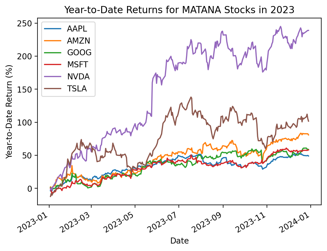
1.2 The pandas-datareader package
The pandas-datareader package provides easy access to various data sources, including the Kenneth French Data Library and the Federal Reserve Economic Data (FRED). The pandas-datareader package also downloads Yahoo! Finance data, but the yfinance package has better documentation. We will use pdr as the abbreviated prefix for pandas-datareader.
import pandas_datareader as pdrHere we download the daily benchmark factors from Ken French’s Data Library.
pdr.famafrench.get_available_datasets()[:5]['F-F_Research_Data_Factors',
'F-F_Research_Data_Factors_weekly',
'F-F_Research_Data_Factors_daily',
'F-F_Research_Data_5_Factors_2x3',
'F-F_Research_Data_5_Factors_2x3_daily']For Fama and French data, pandas-datareader returns the most recent five years of data unless we specify a start date. French typically provides data back through the second half of 1926. pandas-datareader returns dictionaries of data frames, and the 'DESCR' value describes these data frames.
ff_all = pdr.DataReader(
    name='F-F_Research_Data_Factors_daily',
    data_source='famafrench',
    start='1900'
)
C:\Users\r.herron\AppData\Local\Temp\ipykernel_26796\2526882917.py:1: FutureWarning: The argument 'date_parser' is deprecated and will be removed in a future version. Please use 'date_format' instead, or read your data in as 'object' dtype and then call 'to_datetime'.
ff_all = pdr.DataReader(type(ff_all)dictprint(ff_all['DESCR'])F-F Research Data Factors daily
-------------------------------
This file was created by CMPT_ME_BEME_RETS_DAILY using the 202312 CRSP database. The Tbill return is the simple daily rate that, over the number of trading days in the month, compounds to 1-month TBill rate from Ibbotson and Associates Inc. Copyright 2023 Kenneth R. French
0 : (25649 rows x 4 cols)ff_all[0]| Mkt-RF | SMB | HML | RF | |
|---|---|---|---|---|
| Date | ||||
| 1926-07-01 | 0.1000 | -0.2500 | -0.2700 | 0.0090 |
| 1926-07-02 | 0.4500 | -0.3300 | -0.0600 | 0.0090 |
| 1926-07-06 | 0.1700 | 0.3000 | -0.3900 | 0.0090 |
| 1926-07-07 | 0.0900 | -0.5800 | 0.0200 | 0.0090 |
| 1926-07-08 | 0.2100 | -0.3800 | 0.1900 | 0.0090 |
| ... | ... | ... | ... | ... |
| 2023-12-22 | 0.2100 | 0.6400 | 0.0900 | 0.0210 |
| 2023-12-26 | 0.4800 | 0.6900 | 0.4600 | 0.0210 |
| 2023-12-27 | 0.1600 | 0.1400 | 0.1200 | 0.0210 |
| 2023-12-28 | -0.0100 | -0.3600 | 0.0300 | 0.0210 |
| 2023-12-29 | -0.4300 | -1.1200 | -0.3700 | 0.0210 |
25649 rows × 4 columns
(
    ff_all[0] # slice factors
    .div(100) # convert to decimal
    .add(1) # calculate cumulative returns
    .cumprod()
    .sub(1)
    .mul(100) # convert to percent
    .plot() # plot
)
plt.ylabel('Cumulative Return (%)')
plt.title('Cumulative Returns for the Daily Benchmark Factors')
plt.gca().yaxis.set_major_formatter(plt.matplotlib.ticker.StrMethodFormatter('{x:,.0f}'))
# plt.yscale('log') # log scale impractical here with negative returns
plt.show()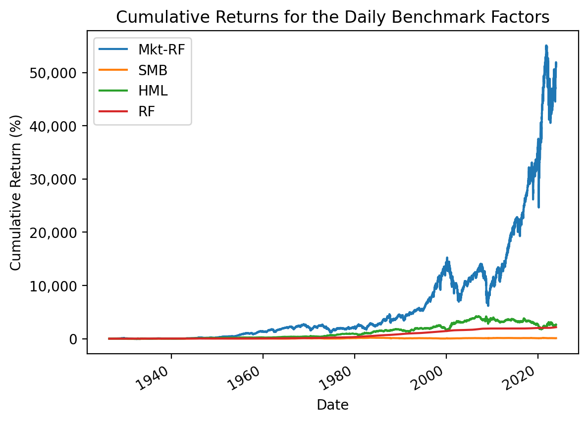
2 Log and Simple Returns
We will typically use simple returns, calculated as \(R_{simple,t} = \frac{P_t + D_t - P_{t-1}}{P_{t-1}} = \frac{P_t + D_t}{P_{t-1}} - 1\). The simple return is the return that investors receive on invested dollars. We can calculate simple returns from Yahoo Finance data with the .pct_change() method on the adjusted close column (i.e., Adj Close), which adjusts for dividends and splits. The adjusted close column is a reverse-engineered close price (i.e., end-of-trading-day price) that incorporates dividends and splits, making simple return calculations easy.
However, we may see log returns elsewhere, which are the (natural) log of one plus simple returns: \[R_{log,t} = \log(1 + R_{simple,t}) = \log\left(1 + \frac{P_t + D_t}{P_{t-1}} - 1 \right) = \log\left(\frac{P_t + D_t}{P_{t-1}} \right) = \log(P_t + D_t) - \log(P_{t-1})\] Therefore, we calculate log returns as either the log of one plus simple returns or the difference of the logs of the adjusted close column. Log returns are also known as continuously-compounded returns.
We will typically use simple returns instead of log returns. However, this section explains the differences between simple and log returns and where each is appropriate.
2.1 Simple and Log Returns are Similar for Small Returns
\(\log(1 + x) \approx x\) for small values of \(x\), so simple returns and log returns are similar for small returns. Returns are typically small at daily and monthly horizons, so the difference between simple and log returns is small at these horizons. The following figure shows \(R_{simple,t} \approx R_{log,t}\) for small \(R\)s.
R = np.linspace(-0.75, 0.75, 100)
logR = np.log(1 + R)
plt.plot(R, logR)
plt.plot([-1, 1], [-1, 1])
plt.xlabel('Simple Return')
plt.ylabel('Log Return')
plt.title('Log Versus Simple Returns')
plt.legend(['Actual', 'If Log = Simple'])
plt.show()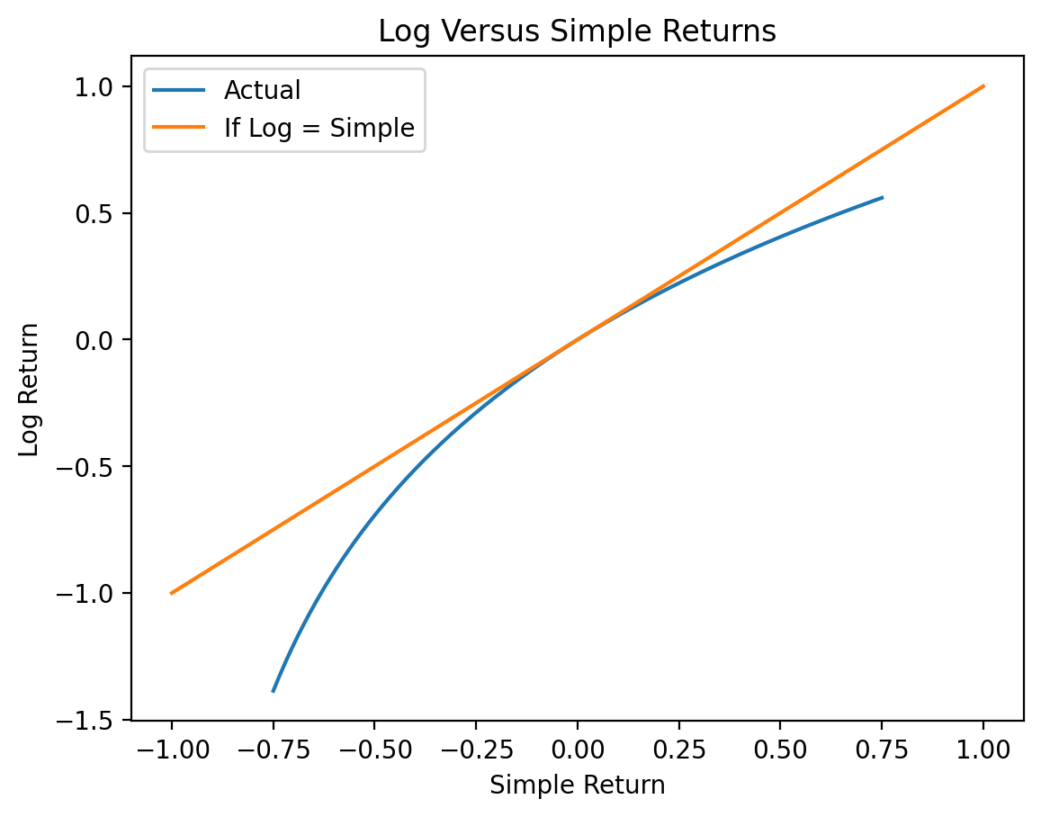
2.2 Simple Return Advantage: Portfolio Calculations
We can only perform portfolio calculations with simple returns. For a portfolio of \(N\) assets with portfolio weights \(w_i\), the portfolio return \(R_{p}\) is the weighted average of the returns of its assets, \(R_{p} = \sum_{i=1}^N w_i R_{i}\). For two stocks with portfolio weights of 50%, our portfolio return is \(R_{portfolio} = 0.5 R_1 + 0.5 R_2 = \frac{R_1 + R_2}{2}\). However, we cannot calculate portfolio returns with log returns because the sum of logs is the log of products.
We cannot calculate portfolio returns as the weighted average of log returns.
2.3 Log Return Advantage: Log Returns are Additive
The advantage of log returns is that we can compound log returns with addition. The additive property of log returns makes code simple, computations fast, and proofs easy when we compound returns over multiple periods.
We compound returns from \(t=0\) to \(t=T\) as follows: \[1 + R_{0, T} = (1 + R_1) \times (1 + R_2) \times \dots \times (1 + R_T)\]
Next, we take the log of both sides of the previous equation and use the property that the log of products is the sum of logs: \[\log(1 + R_{0, T}) = \log((1 + R_1) \times (1 + R_2) \times \dots \times (1 + R_T)) = \log(1 + R_1) + \log(1 + R_2) + \dots + \log(1 + R_T) = \sum_{t=1}^T \log(1 + R_t)\]
Next, we exponentiate both sides of the previous equation: \[e^{\log(1 + R_{0, T})} = e^{\sum_{t=0}^T \log(1 + R_t)}\]
Next, we use the property that \(e^{\log(x)} = x\) to simplify the previous equation: \[1 + R_{0,T} = e^{\sum_{t=0}^T \log(1 + R_t)}\]
Finally, we subtract 1 from both sides: \[R_{0 ,T} = e^{\sum_{t=0}^T \log(1 + R_t)} - 1\]
So, the return \(R_{0,T}\) from \(t=0\) to \(t=T\) is the exponentiated sum of log returns. The pandas developers assume users understand the math above and focus on optimizing sums.
The following code generates 10,000 random log returns. The np.random.randn() call generates normally distributed random numbers. To generate equivalent simple returns, we exponentiate these log returns, then subtract one.
np.random.seed(42)
df2 = pd.DataFrame(data={'R': np.exp(np.random.randn(10000)) - 1})
df2| R | |
|---|---|
| 0 | 0.6433 |
| 1 | -0.1291 |
| 2 | 0.9111 |
| 3 | 3.5861 |
| 4 | -0.2088 |
| ... | ... |
| 9995 | 2.6733 |
| 9996 | -0.8644 |
| 9997 | -0.5060 |
| 9998 | 0.6418 |
| 9999 | 0.9048 |
10000 rows × 1 columns
df2.describe()| R | |
|---|---|
| count | 10000.0000 |
| mean | 0.6529 |
| std | 2.1918 |
| min | -0.9802 |
| 25% | -0.4896 |
| 50% | -0.0026 |
| 75% | 0.9564 |
| max | 49.7158 |
We can time the calculation of 12-observation rolling returns. We use .apply() for the simple return version because .rolling() does not have a product method. We find that .rolling() is slower with .apply() than with .sum() by a factor of 2,000. We will learn about .rolling() and .apply() in a few weeks, but they provide the best example of when to use log returns.
%%timeit
df2['R12_via_simple'] = (
    df2['R']
    .add(1)
    .rolling(12)
    .apply(lambda x: x.prod())
    .sub(1)
)
284 ms ± 80.7 ms per loop (mean ± std. dev. of 7 runs, 1 loop each)%%timeit
df2['R12_via_log'] = (
df2['R']
.add(1)
.pipe(np.log)
.rolling(12)
.sum()
.pipe(np.exp)
.sub(1)
)557 µs ± 60.6 µs per loop (mean ± std. dev. of 7 runs, 1,000 loops each)df2.head(15)| R | R12_via_simple | R12_via_log | |
|---|---|---|---|
| 0 | 0.6433 | NaN | NaN |
| 1 | -0.1291 | NaN | NaN |
| 2 | 0.9111 | NaN | NaN |
| 3 | 3.5861 | NaN | NaN |
| 4 | -0.2088 | NaN | NaN |
| 5 | -0.2087 | NaN | NaN |
| 6 | 3.8511 | NaN | NaN |
| 7 | 1.1542 | NaN | NaN |
| 8 | -0.3747 | NaN | NaN |
| 9 | 0.7204 | NaN | NaN |
| 10 | -0.3709 | NaN | NaN |
| 11 | -0.3723 | 33.8643 | 33.8643 |
| 12 | 0.2737 | 26.0236 | 26.0236 |
| 13 | -0.8524 | 3.5800 | 3.5800 |
| 14 | -0.8218 | -0.5730 | -0.5730 |
np.allclose(df2['R12_via_simple'], df2['R12_via_log'], equal_nan=True)TrueThese two approaches calculate the same return, but the simple-return approach is 1,000 times slower than the log-return approach!
We can use log returns to calculate total returns very quickly!
3 Portfolio Math
Portfolio return \(R_{p}\) is the weighted average of its asset returns, so \(R_{p} = \sum_{i=1}^N w_i R_{i}\). Here \(N\) is the number of assets, and \(w_i\) is the weight on asset \(i\).
3.1 The 1/N Portfolio
The \(\frac{1}{N}\) portfolio equally weights portfolio assets, so \(w_1 = w_2 = \dots = w_N = \frac{1}{N}\). We typically rebalance the \(\frac{1}{N}\) portfolio every period. If \(w_i = \frac{1}{N}\), then \(R_{p} = \sum_{i=1}^N \frac{1}{N} R_{i} = \frac{\sum_{i=1}^N R_i}{N} = \bar{R}\). Therefore, we can use .mean() to calculate \(\frac{1}{N}\) portfolio returns.
returns = df['Adj Close'].pct_change().loc['2023']

returns| AAPL | AMZN | GOOG | MSFT | NVDA | TSLA | |
|---|---|---|---|---|---|---|
| Date | ||||||
| 2023-01-03 | -0.0374 | 0.0217 | 0.0109 | -0.0010 | -0.0205 | -0.1224 |
| 2023-01-04 | 0.0103 | -0.0079 | -0.0110 | -0.0437 | 0.0303 | 0.0512 |
| 2023-01-05 | -0.0106 | -0.0237 | -0.0219 | -0.0296 | -0.0328 | -0.0290 |
| 2023-01-06 | 0.0368 | 0.0356 | 0.0160 | 0.0118 | 0.0416 | 0.0247 |
| 2023-01-09 | 0.0041 | 0.0149 | 0.0073 | 0.0097 | 0.0518 | 0.0593 |
| ... | ... | ... | ... | ... | ... | ... |
| 2023-12-22 | -0.0055 | -0.0027 | 0.0065 | 0.0028 | -0.0033 | -0.0077 |
| 2023-12-26 | -0.0028 | -0.0001 | 0.0007 | 0.0002 | 0.0092 | 0.0161 |
| 2023-12-27 | 0.0005 | -0.0005 | -0.0097 | -0.0016 | 0.0028 | 0.0188 |
| 2023-12-28 | 0.0022 | 0.0003 | -0.0011 | 0.0032 | 0.0021 | -0.0316 |
| 2023-12-29 | -0.0054 | -0.0094 | -0.0025 | 0.0020 | 0.0000 | -0.0186 |
250 rows × 6 columns
returns.mean()AAPL 0.0017
AMZN 0.0026
GOOG 0.0020
MSFT 0.0020
NVDA 0.0053
TSLA 0.0034
dtype: float64rp_1 = returns.mean(axis=1)
rp_1Date
2023-01-03 -0.0248
2023-01-04 0.0049
2023-01-05 -0.0246
2023-01-06 0.0278
2023-01-09 0.0245
...
2023-12-22 -0.0017
2023-12-26 0.0039
2023-12-27 0.0017
2023-12-28 -0.0041
2023-12-29 -0.0056
Length: 250, dtype: float64Note that when we apply the same portfolio weights every period, we rebalance at the same frequency as the returns data. If we have daily data, rebalance daily. If we have monthly data, we rebalance monthly, and so on.
3.2 A More General Solution
If we combine weights into vector \(w\) and the time series of asset returns into matrix \(\mathbf{R}\), then we can calculate the time series of portfolio returns as \(R_p = w^T \mathbf{R}\). The pandas version of this calculation is R.dot(w), where R is a data frame of asset returns and w is a series of portfolio weights. We can use this approach to calculate \(\frac{1}{N}\) portfolio returns, too.
weights = np.ones(returns.shape[1]) / returns.shape[1]
weights
array([0.1667, 0.1667, 0.1667, 0.1667, 0.1667, 0.1667])rp_2 = returns.dot(weights)
rp_2Date
2023-01-03 -0.0248
2023-01-04 0.0049
2023-01-05 -0.0246
2023-01-06 0.0278
2023-01-09 0.0245
...
2023-12-22 -0.0017
2023-12-26 0.0039
2023-12-27 0.0017
2023-12-28 -0.0041
2023-12-29 -0.0056
Length: 250, dtype: float64Both approaches give the same answer!
np.allclose(rp_1, rp_2, equal_nan=True)True