import matplotlib.pyplot as plt
import numpy as np
import pandas as pd
import pandas_datareader as pdr
import yfinance as yfMcKinney Chapter 8 - Practice for Section 04
FINA 6333 for Spring 2024
1 Announcements
- Joining Data with pandas, our fourth and final DataCamp course, is due by Friday, 2/16, at 11:59 PM
- We will use class next week, from 2/19 through 2/23, for group work on Project 1, so there is no lecture video or pre-class quiz
- Project 1 is due by Tuesday, 2/27, at 8:25 AM
- Please complete the anonymous ungraded survey on Canvas to help me help you learn better:
2 10-Minute Recap
Chapter 8 of McKinney covers 3 topics.
- Hierarchical Indexing: Hierarchical indexing helps us organize data at multiple levels, rather than just a flat, two-dimensional structure. It helps is work with high-dimensional data in a low-dimensional form. For example, we can index rows by multiple levels like “ticker” and “date”, or columns by “variable” and “ticker”.
- Combining Data: We can combine datasets on one or more keys.
- We will use the
pd.merge()function for database-style joins, which can beinner,outer,left, orrightjoins. - We will use the
.join()method to combine data frames with similar indexes. - We will use the
pd.concat()to combine similarly-shaped series and data frames.
- We will use the
- Reshaping Data: We can reshape data to change its structure, such as pivoting from wide to long format or vice versa. We will most often use the
.stack()and.unstack()methods, which pivot columns to rows and rows to columns, respectively. Laster in the course we will learn about the.pivot()method for aggregating data and the.melt()method for more advanced reshaping.
3 Practice
%precision 4
pd.options.display.float_format = '{:.4f}'.format
%config InlineBackend.figure_format = 'retina'
3.1 Download data from Yahoo! Finance for BAC, C, GS, JPM, MS, and PNC and assign to data frame stocks.
Use .rename_axis(columns=stocks.columns.names = ['Variable', 'Ticker']) to assign the names Variable and Ticker to the column multi index. We could instead use stocks.columns.names = ['Variable', 'Ticker'], but we can chain the .rename_axis() method.
stocks = (
    yf.download(tickers='BAC C GS JPM MS PNC')
    .rename_axis(columns=['Variable', 'Ticker'])
)
[*********************100%%**********************] 6 of 6 completedstocks.tail()| Variable | Adj Close | Close | ... | Open | Volume | ||||||||||||||||
|---|---|---|---|---|---|---|---|---|---|---|---|---|---|---|---|---|---|---|---|---|---|
| Ticker | BAC | C | GS | JPM | MS | PNC | BAC | C | GS | JPM | ... | GS | JPM | MS | PNC | BAC | C | GS | JPM | MS | PNC |
| Date | |||||||||||||||||||||
| 2024-02-12 | 33.6200 | 53.9200 | 392.6400 | 175.7900 | 86.8700 | 149.1400 | 33.6200 | 53.9200 | 392.6400 | 175.7900 | ... | 385.0000 | 174.7800 | 85.8600 | 147.7700 | 34160400 | 17162300.0000 | 2797200.0000 | 8539300.0000 | 7888000.0000 | 1612700.0000 |
| 2024-02-13 | 32.7500 | 52.7600 | 378.7500 | 174.2600 | 83.9700 | 145.2600 | 32.7500 | 52.7600 | 378.7500 | 174.2600 | ... | 387.5900 | 175.3200 | 85.8600 | 146.7800 | 43801500 | 17672100.0000 | 3030800.0000 | 8397600.0000 | 11339400.0000 | 2121400.0000 |
| 2024-02-14 | 33.1300 | 53.9800 | 378.0400 | 176.0300 | 84.0000 | 147.8700 | 33.1300 | 53.9800 | 378.0400 | 176.0300 | ... | 380.8800 | 175.0700 | 84.5400 | 146.6300 | 27833900 | 14891900.0000 | 2041300.0000 | 7056700.0000 | 5973700.0000 | 1265300.0000 |
| 2024-02-15 | 34.0700 | 55.2100 | 385.4200 | 179.8700 | 85.6700 | 149.6300 | 34.0700 | 55.2100 | 385.4200 | 179.8700 | ... | 379.4200 | 176.1500 | 84.4500 | 148.7500 | 41683100 | 16865000.0000 | 2218900.0000 | 8723400.0000 | 7993500.0000 | 1991800.0000 |
| 2024-02-16 | 34.0900 | 54.8500 | 384.4400 | 179.0300 | 86.5000 | 148.8500 | 34.0900 | 54.8500 | 384.4400 | 179.0300 | ... | 383.2400 | 179.6100 | 85.5200 | 148.4200 | 33146357 | 11419637.0000 | 2302099.0000 | 7927785.0000 | 9628557.0000 | 1362728.0000 |
5 rows × 36 columns
3.2 Reshape stocks from wide to long with dates and tickers as row indexes and assign to data frame stocks_long.
By default, .stack() stacks the inner column index to the inner row index.
stocks_long = stocks.stack()stocks_long.tail()| Variable | Adj Close | Close | High | Low | Open | Volume | |
|---|---|---|---|---|---|---|---|
| Date | Ticker | ||||||
| 2024-02-16 | C | 54.8500 | 54.8500 | 55.1950 | 54.5500 | 54.9600 | 11419637.0000 |
| GS | 384.4400 | 384.4400 | 387.5800 | 380.9450 | 383.2400 | 2302099.0000 | |
| JPM | 179.0300 | 179.0300 | 179.9800 | 178.1600 | 179.6100 | 7927785.0000 | |
| MS | 86.5000 | 86.5000 | 86.7900 | 85.0700 | 85.5200 | 9628557.0000 | |
| PNC | 148.8500 | 148.8500 | 149.9100 | 147.6900 | 148.4200 | 1362728.0000 |
3.3 Add daily returns for each stock to data frames stocks and stocks_long.
Name the returns variable Returns, and maintain all multi indexes. Hint: Use pd.MultiIndex() to create a multi index for the the wide data frame stocks.
stocks['Adj Close'].columnsIndex(['BAC', 'C', 'GS', 'JPM', 'MS', 'PNC'], dtype='object', name='Ticker')_ = pd.MultiIndex.from_product([['Returns'], stocks['Adj Close'].columns])
stocks[_] = stocks['Adj Close'].iloc[:-1].pct_change()stocks.tail()| Variable | Adj Close | Close | ... | Volume | Returns | ||||||||||||||||
|---|---|---|---|---|---|---|---|---|---|---|---|---|---|---|---|---|---|---|---|---|---|
| Ticker | BAC | C | GS | JPM | MS | PNC | BAC | C | GS | JPM | ... | GS | JPM | MS | PNC | BAC | C | GS | JPM | MS | PNC |
| Date | |||||||||||||||||||||
| 2024-02-12 | 33.6200 | 53.9200 | 392.6400 | 175.7900 | 86.8700 | 149.1400 | 33.6200 | 53.9200 | 392.6400 | 175.7900 | ... | 2797200.0000 | 8539300.0000 | 7888000.0000 | 1612700.0000 | 0.0166 | -0.0013 | 0.0218 | 0.0045 | 0.0114 | 0.0093 |
| 2024-02-13 | 32.7500 | 52.7600 | 378.7500 | 174.2600 | 83.9700 | 145.2600 | 32.7500 | 52.7600 | 378.7500 | 174.2600 | ... | 3030800.0000 | 8397600.0000 | 11339400.0000 | 2121400.0000 | -0.0259 | -0.0215 | -0.0354 | -0.0087 | -0.0334 | -0.0260 |
| 2024-02-14 | 33.1300 | 53.9800 | 378.0400 | 176.0300 | 84.0000 | 147.8700 | 33.1300 | 53.9800 | 378.0400 | 176.0300 | ... | 2041300.0000 | 7056700.0000 | 5973700.0000 | 1265300.0000 | 0.0116 | 0.0231 | -0.0019 | 0.0102 | 0.0004 | 0.0180 |
| 2024-02-15 | 34.0700 | 55.2100 | 385.4200 | 179.8700 | 85.6700 | 149.6300 | 34.0700 | 55.2100 | 385.4200 | 179.8700 | ... | 2218900.0000 | 8723400.0000 | 7993500.0000 | 1991800.0000 | 0.0284 | 0.0228 | 0.0195 | 0.0218 | 0.0199 | 0.0119 |
| 2024-02-16 | 34.0900 | 54.8500 | 384.4400 | 179.0300 | 86.5000 | 148.8500 | 34.0900 | 54.8500 | 384.4400 | 179.0300 | ... | 2302099.0000 | 7927785.0000 | 9628557.0000 | 1362728.0000 | NaN | NaN | NaN | NaN | NaN | NaN |
5 rows × 42 columns
The easiest way to add returns to long data frame stocks_long is to .stack() the wide data frame stocks! We could sort stocks_long by ticker and date (to sort chronologically within each ticker), then use .pct_change(). However, this approach miscalculates the first return for every ticker except for the first ticker. The easiest and safest solution is to .stack() the wide data frame stocks!
stocks_long = stocks.stack()stocks_long.tail()| Variable | Adj Close | Close | High | Low | Open | Volume | Returns | |
|---|---|---|---|---|---|---|---|---|
| Date | Ticker | |||||||
| 2024-02-16 | C | 54.8500 | 54.8500 | 55.1950 | 54.5500 | 54.9600 | 11419637.0000 | NaN |
| GS | 384.4400 | 384.4400 | 387.5800 | 380.9450 | 383.2400 | 2302099.0000 | NaN | |
| JPM | 179.0300 | 179.0300 | 179.9800 | 178.1600 | 179.6100 | 7927785.0000 | NaN | |
| MS | 86.5000 | 86.5000 | 86.7900 | 85.0700 | 85.5200 | 9628557.0000 | NaN | |
| PNC | 148.8500 | 148.8500 | 149.9100 | 147.6900 | 148.4200 | 1362728.0000 | NaN |
3.4 Download the daily benchmark return factors from Ken French’s data library.
pdr.famafrench.get_available_datasets()[:5]['F-F_Research_Data_Factors',
'F-F_Research_Data_Factors_weekly',
'F-F_Research_Data_Factors_daily',
'F-F_Research_Data_5_Factors_2x3',
'F-F_Research_Data_5_Factors_2x3_daily']ff = (
pdr.DataReader(
name='F-F_Research_Data_Factors_daily',
data_source='famafrench',
start='1900'
)
[0]
.div(100)
)C:\Users\r.herron\AppData\Local\Temp\ipykernel_4188\2049483829.py:2: FutureWarning: The argument 'date_parser' is deprecated and will be removed in a future version. Please use 'date_format' instead, or read your data in as 'object' dtype and then call 'to_datetime'.
pdr.DataReader(ff.tail()| Mkt-RF | SMB | HML | RF | |
|---|---|---|---|---|
| Date | ||||
| 2023-12-22 | 0.0021 | 0.0064 | 0.0009 | 0.0002 |
| 2023-12-26 | 0.0048 | 0.0069 | 0.0046 | 0.0002 |
| 2023-12-27 | 0.0016 | 0.0014 | 0.0012 | 0.0002 |
| 2023-12-28 | -0.0001 | -0.0036 | 0.0003 | 0.0002 |
| 2023-12-29 | -0.0043 | -0.0112 | -0.0037 | 0.0002 |
3.5 Add the daily benchmark return factors to stocks and stocks_long.
For the wide data frame stocks, use the outer index name Factors.
# stocks.join(ff)
# MergeError: Not allowed to merge between different levels. (2 levels on the left, 1 on the right)
_ = pd.MultiIndex.from_product([['Factors'], ff.columns])
stocks[_] = ffstocks| Variable | Adj Close | Close | ... | Returns | Factors | ||||||||||||||||
|---|---|---|---|---|---|---|---|---|---|---|---|---|---|---|---|---|---|---|---|---|---|
| Ticker | BAC | C | GS | JPM | MS | PNC | BAC | C | GS | JPM | ... | BAC | C | GS | JPM | MS | PNC | Mkt-RF | SMB | HML | RF |
| Date | |||||||||||||||||||||
| 1973-02-21 | 1.5818 | NaN | NaN | NaN | NaN | NaN | 4.6250 | NaN | NaN | NaN | ... | NaN | NaN | NaN | NaN | NaN | NaN | -0.0074 | -0.0039 | 0.0054 | 0.0002 |
| 1973-02-22 | 1.5872 | NaN | NaN | NaN | NaN | NaN | 4.6406 | NaN | NaN | NaN | ... | 0.0034 | NaN | NaN | NaN | NaN | NaN | -0.0030 | -0.0037 | 0.0022 | 0.0002 |
| 1973-02-23 | 1.5818 | NaN | NaN | NaN | NaN | NaN | 4.6250 | NaN | NaN | NaN | ... | -0.0034 | NaN | NaN | NaN | NaN | NaN | -0.0108 | -0.0019 | 0.0054 | 0.0002 |
| 1973-02-26 | 1.5818 | NaN | NaN | NaN | NaN | NaN | 4.6250 | NaN | NaN | NaN | ... | 0.0000 | NaN | NaN | NaN | NaN | NaN | -0.0088 | -0.0050 | 0.0054 | 0.0002 |
| 1973-02-27 | 1.5818 | NaN | NaN | NaN | NaN | NaN | 4.6250 | NaN | NaN | NaN | ... | 0.0000 | NaN | NaN | NaN | NaN | NaN | -0.0115 | -0.0018 | 0.0064 | 0.0002 |
| ... | ... | ... | ... | ... | ... | ... | ... | ... | ... | ... | ... | ... | ... | ... | ... | ... | ... | ... | ... | ... | ... |
| 2024-02-12 | 33.6200 | 53.9200 | 392.6400 | 175.7900 | 86.8700 | 149.1400 | 33.6200 | 53.9200 | 392.6400 | 175.7900 | ... | 0.0166 | -0.0013 | 0.0218 | 0.0045 | 0.0114 | 0.0093 | NaN | NaN | NaN | NaN |
| 2024-02-13 | 32.7500 | 52.7600 | 378.7500 | 174.2600 | 83.9700 | 145.2600 | 32.7500 | 52.7600 | 378.7500 | 174.2600 | ... | -0.0259 | -0.0215 | -0.0354 | -0.0087 | -0.0334 | -0.0260 | NaN | NaN | NaN | NaN |
| 2024-02-14 | 33.1300 | 53.9800 | 378.0400 | 176.0300 | 84.0000 | 147.8700 | 33.1300 | 53.9800 | 378.0400 | 176.0300 | ... | 0.0116 | 0.0231 | -0.0019 | 0.0102 | 0.0004 | 0.0180 | NaN | NaN | NaN | NaN |
| 2024-02-15 | 34.0700 | 55.2100 | 385.4200 | 179.8700 | 85.6700 | 149.6300 | 34.0700 | 55.2100 | 385.4200 | 179.8700 | ... | 0.0284 | 0.0228 | 0.0195 | 0.0218 | 0.0199 | 0.0119 | NaN | NaN | NaN | NaN |
| 2024-02-16 | 34.0900 | 54.8500 | 384.4400 | 179.0300 | 86.5000 | 148.8500 | 34.0900 | 54.8500 | 384.4400 | 179.0300 | ... | NaN | NaN | NaN | NaN | NaN | NaN | NaN | NaN | NaN | NaN |
12860 rows × 46 columns
stocks_long = stocks_long.join(ff)stocks_long.loc['2023'].tail(12)| Adj Close | Close | High | Low | Open | Volume | Returns | Mkt-RF | SMB | HML | RF | ||
|---|---|---|---|---|---|---|---|---|---|---|---|---|
| Date | Ticker | |||||||||||
| 2023-12-28 | BAC | 33.8800 | 33.8800 | 33.9700 | 33.7700 | 33.8200 | 21799600.0000 | 0.0012 | -0.0001 | -0.0036 | 0.0003 | 0.0002 |
| C | 51.0329 | 51.5200 | 51.8000 | 51.4000 | 51.4000 | 10218500.0000 | 0.0012 | -0.0001 | -0.0036 | 0.0003 | 0.0002 | |
| GS | 386.4100 | 386.4100 | 387.7600 | 383.6300 | 384.5200 | 1024700.0000 | 0.0050 | -0.0001 | -0.0036 | 0.0003 | 0.0002 | |
| JPM | 169.2563 | 170.3000 | 170.6600 | 169.0000 | 169.3500 | 6320100.0000 | 0.0053 | -0.0001 | -0.0036 | 0.0003 | 0.0002 | |
| MS | 92.7316 | 93.6400 | 93.9500 | 93.2400 | 93.3100 | 4089500.0000 | -0.0002 | -0.0001 | -0.0036 | 0.0003 | 0.0002 | |
| PNC | 154.0486 | 155.6300 | 156.2100 | 154.9500 | 155.4400 | 1153300.0000 | 0.0041 | -0.0001 | -0.0036 | 0.0003 | 0.0002 | |
| 2023-12-29 | BAC | 33.6700 | 33.6700 | 33.9900 | 33.5500 | 33.9400 | 28037800.0000 | -0.0062 | -0.0043 | -0.0112 | -0.0037 | 0.0002 |
| C | 50.9537 | 51.4400 | 51.6100 | 51.2200 | 51.5600 | 13147900.0000 | -0.0016 | -0.0043 | -0.0112 | -0.0037 | 0.0002 | |
| GS | 385.7700 | 385.7700 | 386.6400 | 383.5700 | 385.5700 | 881300.0000 | -0.0017 | -0.0043 | -0.0112 | -0.0037 | 0.0002 | |
| JPM | 169.0575 | 170.1000 | 170.6900 | 169.6300 | 170.0000 | 6431800.0000 | -0.0012 | -0.0043 | -0.0112 | -0.0037 | 0.0002 | |
| MS | 92.3454 | 93.2500 | 93.7700 | 93.0600 | 93.4900 | 4772100.0000 | -0.0042 | -0.0043 | -0.0112 | -0.0037 | 0.0002 | |
| PNC | 153.2765 | 154.8500 | 156.1100 | 154.5200 | 155.2700 | 1572600.0000 | -0.0050 | -0.0043 | -0.0112 | -0.0037 | 0.0002 |
3.6 Write a function download() that accepts tickers and returns a wide data frame of returns with the daily benchmark return factors.
We can even add a shape argument to return a wide or long data frame!
def download(tickers, shape='wide'):
    if shape.lower() not in ['wide', 'long']:
        raise ValueError('Invalid shape: must be "wide" or "long".')

    stocks = yf.download(tickers)

    factors_all = (
        pdr.DataReader(
            name='F-F_Research_Data_Factors_daily',
            data_source='famafrench',
            start='1900'
        )
    )

    factors = factors_all[0].div(100)

    # if stocks has a multi index on the columns because we asked for more than one ticker
    # then we have more work to do
    if type(stocks.columns) is pd.MultiIndex:

        # whether we want a wide or long data frame, it is easier to add returns to a wide data frame
        _ = pd.MultiIndex.from_product([['Returns'], stocks['Adj Close'].columns])
        stocks[_] = stocks['Adj Close'].pct_change()

        # if we want a wide data frame, then we need a factors multi index
        if shape.lower() == 'wide':
            _ = pd.MultiIndex.from_product([['Factors'], factors.columns])
            stocks[_] = factors
            return stocks.rename_axis(columns=['Variable', 'Ticker'])

        # if we want a long data frame, then we need to stack stocks and join factors
        # because we tested for wide and long above, we know that here shape must be long
        else:
            return stocks.stack().join(factors).rename_axis(columns=['Variable'], index=['Date', 'Ticker'])

    # if stocks does not have a multi index on the columns
    # then we only have join factors
    else:
return stocks.join(ff).rename_axis(columns=['Variable'])download(tickers=['AAPL', 'TSLA'], shape='long')[*********************100%%**********************] 2 of 2 completed
C:\Users\r.herron\AppData\Local\Temp\ipykernel_4188\3667605341.py:8: FutureWarning: The argument 'date_parser' is deprecated and will be removed in a future version. Please use 'date_format' instead, or read your data in as 'object' dtype and then call 'to_datetime'.
pdr.DataReader(| Variable | Adj Close | Close | High | Low | Open | Volume | Returns | Mkt-RF | SMB | HML | RF | |
|---|---|---|---|---|---|---|---|---|---|---|---|---|
| Date | Ticker | |||||||||||
| 1980-12-12 | AAPL | 0.0992 | 0.1283 | 0.1289 | 0.1283 | 0.1283 | 469033600.0000 | NaN | 0.0138 | -0.0001 | -0.0105 | 0.0006 |
| 1980-12-15 | AAPL | 0.0940 | 0.1217 | 0.1222 | 0.1217 | 0.1222 | 175884800.0000 | -0.0522 | 0.0011 | 0.0025 | -0.0046 | 0.0006 |
| 1980-12-16 | AAPL | 0.0871 | 0.1127 | 0.1133 | 0.1127 | 0.1133 | 105728000.0000 | -0.0734 | 0.0071 | -0.0075 | -0.0047 | 0.0006 |
| 1980-12-17 | AAPL | 0.0893 | 0.1155 | 0.1161 | 0.1155 | 0.1155 | 86441600.0000 | 0.0248 | 0.0152 | -0.0086 | -0.0034 | 0.0006 |
| 1980-12-18 | AAPL | 0.0919 | 0.1189 | 0.1194 | 0.1189 | 0.1189 | 73449600.0000 | 0.0290 | 0.0041 | 0.0022 | 0.0126 | 0.0006 |
| ... | ... | ... | ... | ... | ... | ... | ... | ... | ... | ... | ... | ... |
| 2024-02-14 | TSLA | 188.7100 | 188.7100 | 188.8900 | 183.3500 | 185.3000 | 81203000.0000 | 0.0255 | NaN | NaN | NaN | NaN |
| 2024-02-15 | AAPL | 183.8600 | 183.8600 | 184.4900 | 181.3500 | 183.5500 | 65434500.0000 | -0.0016 | NaN | NaN | NaN | NaN |
| TSLA | 200.4500 | 200.4500 | 200.8800 | 188.8600 | 189.1600 | 120831800.0000 | 0.0622 | NaN | NaN | NaN | NaN | |
| 2024-02-16 | AAPL | 182.3100 | 182.3100 | 184.8500 | 181.6650 | 183.4200 | 48627624.0000 | -0.0084 | NaN | NaN | NaN | NaN |
| TSLA | 199.9500 | 199.9500 | 203.1700 | 197.4000 | 202.0600 | 110528448.0000 | -0.0025 | NaN | NaN | NaN | NaN |
14319 rows × 11 columns
3.8 Combine earnings with the returns from stocks_long.
Use the tz_localize('America/New_York') method add time zone information back to returns.index and use pd.to_timedelta(16, unit='h') to set time to the market close in New York City. Use pd.merge_asof() to match earnings announcement dates and times to appropriate return periods. For example, if a firm announces earnings after the close at 5 PM on February 7, we want to match the return period from 4 PM on February 7 to 4 PM on February 8.
returns = (
    stocks_long
    .reset_index()
    [['Date', 'Ticker', 'Returns']]
    .assign(
        Date=lambda x: x['Date'].dt.tz_localize('America/New_York') + pd.to_timedelta(16, unit='H')
    )
)returns.tail()| Date | Ticker | Returns | |
|---|---|---|---|
| 62021 | 2024-02-16 16:00:00-05:00 | C | NaN |
| 62022 | 2024-02-16 16:00:00-05:00 | GS | NaN |
| 62023 | 2024-02-16 16:00:00-05:00 | JPM | NaN |
| 62024 | 2024-02-16 16:00:00-05:00 | MS | NaN |
| 62025 | 2024-02-16 16:00:00-05:00 | PNC | NaN |
surprises = pd.merge_asof(
    left=earnings.sort_values(['Date', 'Ticker']),
    right=returns.sort_values(['Date', 'Ticker']),
    on='Date',
    by='Ticker',
    direction='forward'
)surprises.tail()| Ticker | Date | EPS Estimate | Reported EPS | Surprise(%) | Returns | |
|---|---|---|---|---|---|---|
| 67 | JPM | 2025-01-15 08:00:00-05:00 | NaN | NaN | NaN | NaN |
| 68 | JPM | 2025-01-15 08:00:00-05:00 | NaN | NaN | NaN | NaN |
| 69 | C | 2025-01-15 11:00:00-05:00 | NaN | NaN | NaN | NaN |
| 70 | PNC | 2025-01-16 08:00:00-05:00 | NaN | NaN | NaN | NaN |
| 71 | PNC | 2025-01-16 10:00:00-05:00 | NaN | NaN | NaN | NaN |
3.9 Plot the relation between daily returns and earnings surprises
Three options in increasing difficulty:
- Scatter plot
- Scatter plot with a best-fit line using
regplot()from the seaborn package - Bar plot using
barplot()from the seaborn package after usingpd.qcut()to form five groups on earnings surprises
(
    surprises
    [['Surprise(%)', 'Returns']]
    .mul(100)
    .plot(kind='scatter', x='Surprise(%)', y='Returns')
)

plt.xlabel('Earnings Surprise (%)')
plt.ylabel('One-Day Return (%)')
plt.title(f'Earnings Surprise Analysis\n {', '.join(tickers.tickers)}')
plt.show()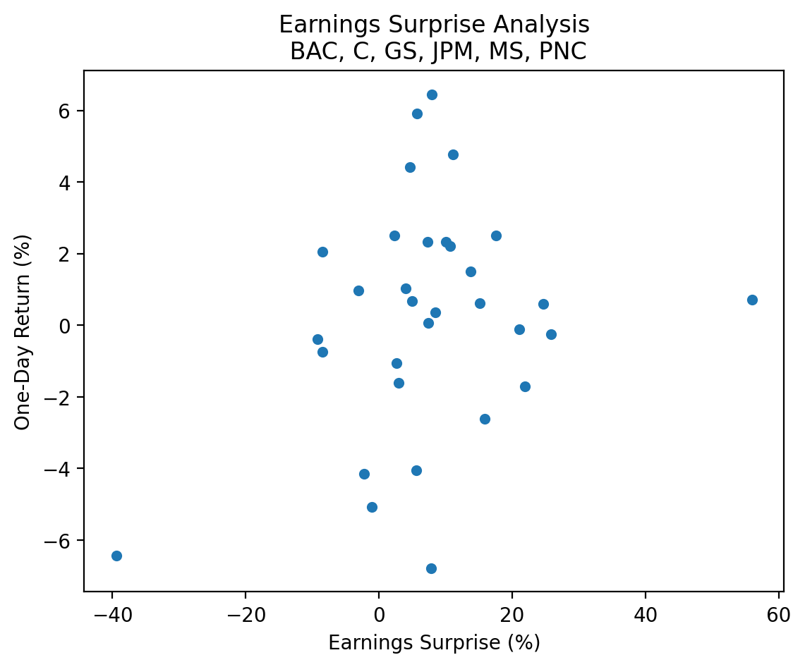
import seaborn as snssns.regplot(
data=surprises[['Surprise(%)', 'Returns']].mul(100),
x='Surprise(%)',
y='Returns'
)
plt.xlabel('Earnings Surprise (%)')
plt.ylabel('One-Day Return (%)')
plt.title(f'Earnings Surprise Analysis\n {', '.join(tickers.tickers)}')
plt.show()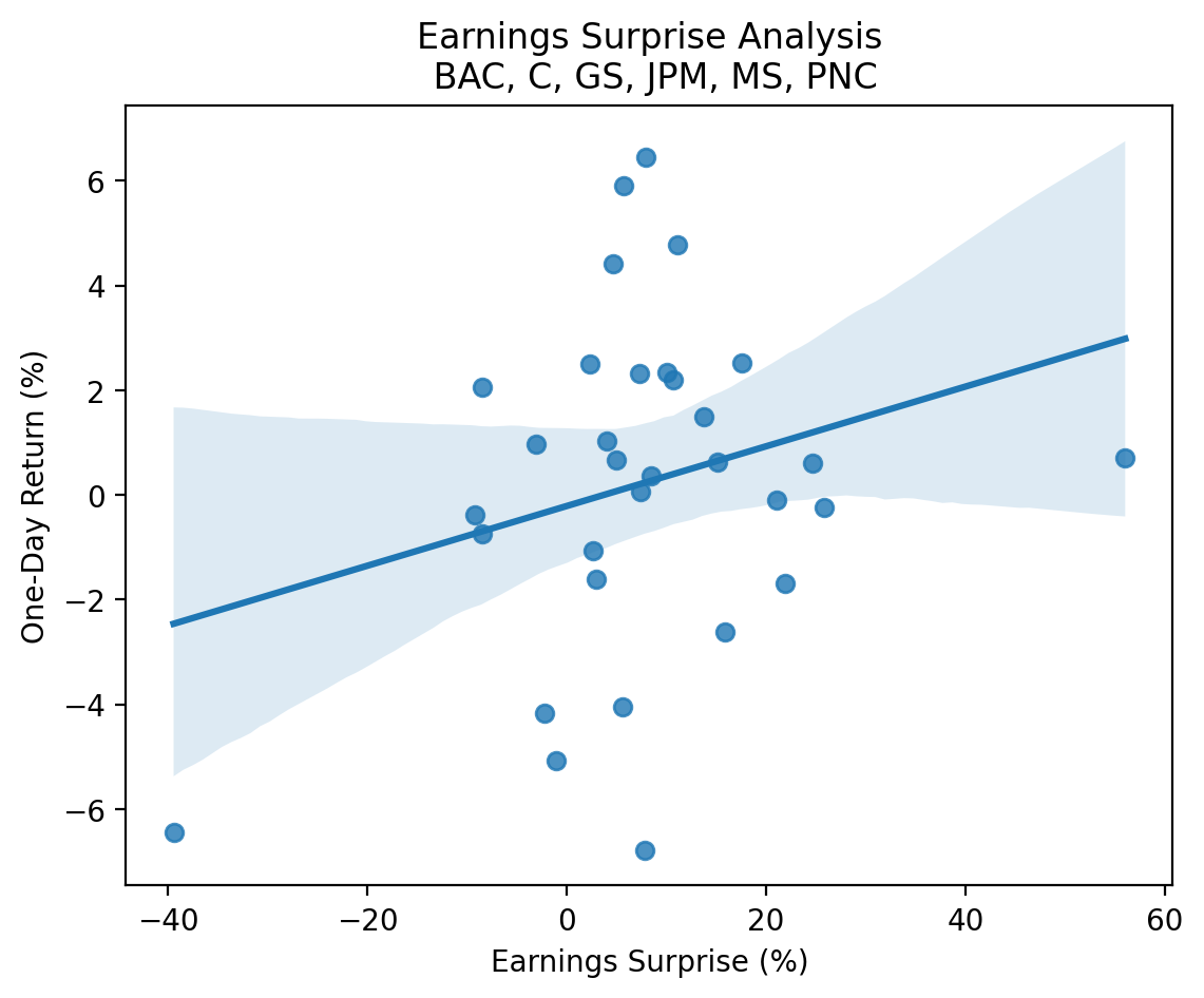
sns.catplot(
    data=(
        surprises[['Surprise(%)', 'Returns']]
        .dropna()
        .mul(100)
        .assign(
            surprise_bin=lambda x: pd.qcut(x['Surprise(%)'], q=5, labels=False)+1
        )
    ),
    x='surprise_bin',
    y='Returns',
    kind='bar'
)

plt.xlabel('Earnings Surprise Bin (1=Lowest, 5=Highest)')
plt.ylabel('One-Day Return (%)')
plt.title(f'Earnings Surprise Analysis\n {', '.join(tickers.tickers)}')
plt.show()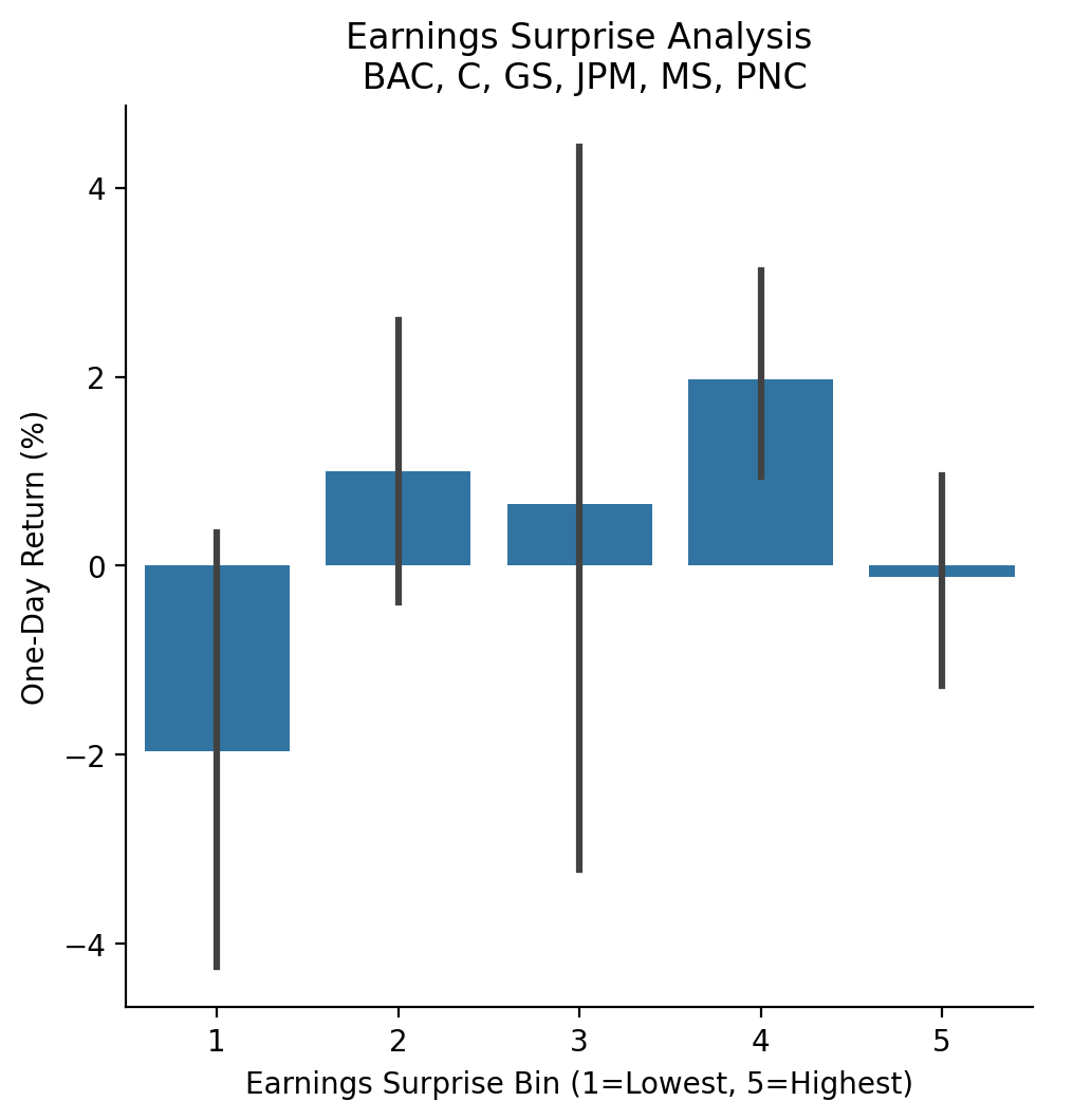
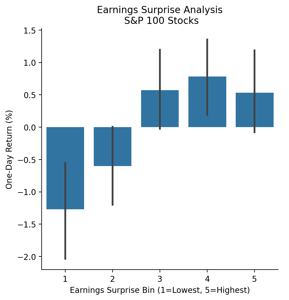
3.10 Repeat the earnings exercise with the S&P 100 stocks
With more data, we can more clearly see the positive relation between earnings surprises and returns!
_ = pd.read_html('https://en.wikipedia.org/wiki/S%26P_100')[2]['Symbol'].to_list()
tickers_2 = yf.Tickers(tickers=[t.replace('.', '-') for t in _]) # Yahoo! Finance uses "-" to indicate share classes instead of "."
earnings_2 = (
pd.concat(
objs=[tickers_2.tickers[t].earnings_dates for t in tickers_2.tickers],
keys=tickers_2.tickers,
names=['Ticker', 'Date']
)
.reset_index()
)earnings_2.tail()| Ticker | Date | EPS Estimate | Reported EPS | Surprise(%) | |
|---|---|---|---|---|---|
| 1207 | XOM | 2023-04-28 06:00:00-04:00 | 2.5900 | 2.8300 | 0.0943 |
| 1208 | XOM | 2023-01-31 06:00:00-05:00 | 3.2900 | 3.4000 | 0.0319 |
| 1209 | XOM | 2022-10-28 06:00:00-04:00 | 3.7900 | 4.4500 | 0.1733 |
| 1210 | XOM | 2022-07-29 06:00:00-04:00 | 3.7400 | 4.1400 | 0.1077 |
| 1211 | XOM | 2022-04-29 06:00:00-04:00 | 2.1200 | 2.0700 | -0.0247 |
returns_2 = (
    yf.download(tickers=[t for t in tickers_2.tickers])
    .rename_axis(columns=['Variable', 'Ticker'])
    ['Adj Close']
    .pct_change()
    .stack()
    .to_frame('Returns')
    .reset_index()
    [['Date', 'Ticker', 'Returns']]
    .assign(
        Date=lambda x: x['Date'].dt.tz_localize('America/New_York') + pd.to_timedelta(16, unit='H')
    )
)
[*********************100%%**********************] 101 of 101 completedreturns_2.tail()| Date | Ticker | Returns | |
|---|---|---|---|
| 1018569 | 2024-02-16 16:00:00-05:00 | V | -0.0086 |
| 1018570 | 2024-02-16 16:00:00-05:00 | VZ | -0.0025 |
| 1018571 | 2024-02-16 16:00:00-05:00 | WFC | -0.0025 |
| 1018572 | 2024-02-16 16:00:00-05:00 | WMT | 0.0063 |
| 1018573 | 2024-02-16 16:00:00-05:00 | XOM | 0.0000 |
surprises_2 = pd.merge_asof(
    left=earnings_2.sort_values(['Date', 'Ticker']),
    right=returns_2.sort_values(['Date', 'Ticker']),
    on='Date',
    by='Ticker',
    direction='forward'
)surprises_2.tail()| Ticker | Date | EPS Estimate | Reported EPS | Surprise(%) | Returns | |
|---|---|---|---|---|---|---|
| 1207 | USB | 2025-10-16 09:00:00-04:00 | NaN | NaN | NaN | NaN |
| 1208 | USB | 2025-10-16 09:00:00-04:00 | NaN | NaN | NaN | NaN |
| 1209 | RTX | 2025-10-20 06:00:00-04:00 | NaN | NaN | NaN | NaN |
| 1210 | USB | 2026-01-20 09:00:00-05:00 | NaN | NaN | NaN | NaN |
| 1211 | USB | 2026-01-20 09:00:00-05:00 | NaN | NaN | NaN | NaN |
(
    surprises_2
    [['Surprise(%)', 'Returns']]
    .mul(100)
    .plot(kind='scatter', x='Surprise(%)', y='Returns')
)

plt.xlabel('Earnings Surprise (%)')
plt.ylabel('One-Day Return (%)')
plt.title('Earnings Surprise Analysis\n S&P 100 Stocks')
plt.show()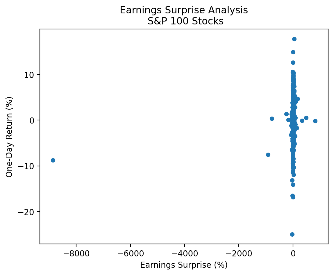
There are a few large negative and positive earnings surprises that make our plot difficult to interpret! We have these huge outliers because surprises are defined as the percent change relative to the expected. If expected is a very small number, then the surprise can be a very large number! We would use different surprise definitions for a more rigorous analysis. Here we can drop observations less than the 0.01 quantile and greater than the 0.99 quantile.
low_2 = surprises_2['Surprise(%)'].quantile(0.01)
high_2 = surprises_2['Surprise(%)'].quantile(0.91)

cond_2 = surprises_2['Surprise(%)'].between(low_2, high_2)
(
surprises_2
.loc[cond_2, ['Surprise(%)', 'Returns']]
.mul(100)
.plot(kind='scatter', x='Surprise(%)', y='Returns', alpha=0.5)
)
plt.xlabel('Earnings Surprise (%)')
plt.ylabel('One-Day Return (%)')
plt.title('Earnings Surprise Analysis\n S&P 100 Stocks')
plt.show()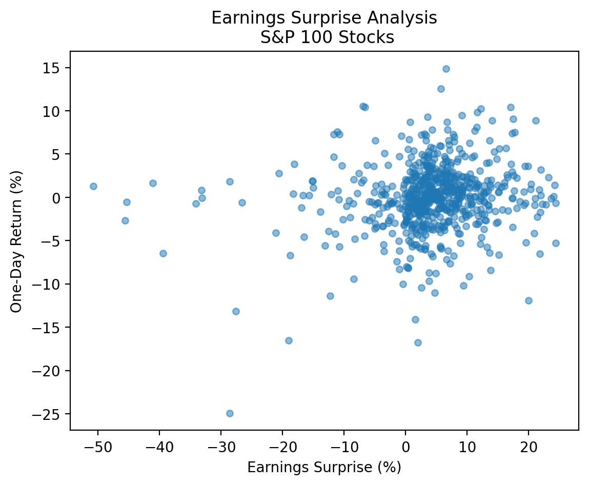
sns.regplot(
    data=surprises_2.loc[cond_2, ['Surprise(%)', 'Returns']].mul(100),
    x='Surprise(%)',
    y='Returns'
)

plt.xlabel('Earnings Surprise (%)')
plt.ylabel('One-Day Return (%)')
plt.title('Earnings Surprise Analysis\n S&P 100 Stocks')
plt.show()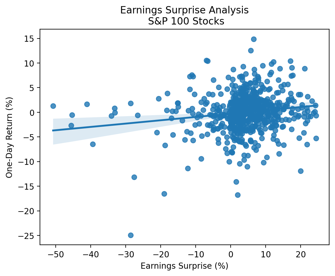
sns.catplot(
    data=(
        surprises_2
        .loc[cond_2, ['Surprise(%)', 'Returns']]
        .dropna()
        .mul(100)
        .assign(surprise_bin=lambda x: pd.qcut(x['Surprise(%)'], q=5, labels=False) + 1)
    ),
    x='surprise_bin',
    y='Returns',
    kind='bar'
)

plt.xlabel('Earnings Surprise Bin (1=Lowest, 5=Highest)')
plt.ylabel('One-Day Return (%)')
plt.title('Earnings Surprise Analysis\n S&P 100 Stocks')
plt.show()