import matplotlib.pyplot as plt
import matplotlib.ticker as ticker
import numpy as np
import pandas as pdProject 3
FINA 6333 for Spring 2025
Purpose
I have two goals for you for this project:
- Implement, backtest, describe, and explain an investing strategy of your choice in Python
- Investigate industry returns; several students have come to me interested in “sector rotation strategies”
Assignment
Use the 49 industry returns to build an investing strategy that maximizes the Sharpe ratio and/or total return. You may use any strategy, such as portfolio optimization, momentum, equal weights, or inverse volatility weights, among others. You may use short weights of up to 30% of your portfolio, including borrowing at the risk-free rate (i.e., RF from the Fama-French factors). You may not use future returns to assemble your current portfolio. That is, for each month, use only past data to set portfolio weights, not future returns.
However, you may backtest your strategy on the full sample, even though this backtesting creates a bias.1 To reduce the impact of this bias, I will backtest all groups on the same random five-year sample.
For my backtest, your notebook must create monthly portfolio returns. Start these returns no later than five years into the sample to allow lookback periods for your strategy. Your notebook must export these returns to a CSV file named Group_XX.csv, where XX is your two-digit group number (e.g., Group_01.csv for Group 01). This CSV file must have only two columns:
Datewith dates in the same format as the Fama-French filesGroup_XX(e.g.,Group_01) with your portfolio returns as decimals
Here is an example row in Group_01.csv: Date,Group_01 with 1931-07,0.0025.
Note
On Friday, 4/11, I added a function to the end of this notebook that you can use export your data for the competition.
I will pick a random five-year period to backtest your strategy and evaluate it based on its Sharpe ratio and total return. The highest Sharpe ratio will earn 15 points, and the highest total return will earn 15 points. Other groups get fewer points based on their Sharpe ratios and total returns relative to the top performers. The other 170 points come from your calculations, visualizations, discussions, and deliverables. See Section 3 and Table 1 for details.
Other important considerations:
- Use only the provided CSV files for industry and factor returns
- Write up to a three-page summary of your strategy, including:
- A description of your strategy
- An explanation of why your strategy might have the highest Sharpe ratio and/or total return
- Figures and tables to support your description and explanation
- Title, label, and caption your figures and tables, referencing them in your summary
Criteria
Table 1 provides the project grading rubric. The project is worth 200 points. The peer reviews are worth 100 points, and students will receive their median score. Almost all students earn perfect peer review scores, so I will factor that into project scores. For example, a project score without peer review scores of \(77.5\%\) converts to a project score with perfect peer review scores of \(85\%\) because \(\frac{0.775 \times 200 + 1.00 \times 100}{300} = 0.85 = 85\%\).
| Topic | Points |
|---|---|
| Clarity, correctness, and completeness of calculations | 50 |
| Clarity, correctness, and completeness of visualizations | 50 |
| Clarity, correctness, and completeness of discussions | 50 |
| Highest Sharpe ratio in the five-year sample that I select | 15 |
| Highest total return in the five-year sample that I select | 15 |
| Correctness of submission according to the deliverables section | 20 |
| Total | 200 |
Deliverables
Upload the following as unzipped files to Canvas by 11:59 PM on 4/23:
- One Jupyter notebook that contains your report, performs all your analysis, and exports a CSV file with your strategy returns
- Name this notebook
project_3.ipynbfor me to run your code - This notebook must run on my computer; I will place the data files in the same folder as your notebook
- Name your exported CSV file
Group_XX.csv, whereXXis your two-digit group number; details are in Section 2
- Name this notebook
- One Quarto-generated Word document with code for me to grade
- Unlike prior projects, submit only one Word document with code
- Name this document
project_3.docx - Use the first cell in this notebook, with
echo: true, to create this Word document with code - You may not edit the Word documents after you create them
Here is some additional guidance:
- Write up to a three-page summary at the start of your report, which is the only writing I will read
- Your submission must not include your name
Data
This project requires two data files. Save these data files as-is in the same folder as your project_3.ipynb notebook file.
data_ind49.csvprovides all available monthly returns from the 49 industries from Kenneth French’s data librarydata_ff3.csvprovides all available monthly returns on the three factors from Kenneth French’s data library
See data_3.ipynb if you want to see how I create these data files. You can read these data files as follows to remove missing values, recreate the PeriodIndex that pdr.DataReader() returns, and convert percent returns to decimal returns.
Note
Several students requested the other Fama-French factors to use a signals. I updated this notebook on Friday, 4/11, to provide two more data files:
data_mom.csvwith the value-weighted monthly returns on the momentum factordata_ff5.csvwith the monthly Fama-French five factors, which only begin in 1963-07 because they require accounting data
ind49 = (
    pd.read_csv(
        filepath_or_buffer='data_ind49.csv',
        parse_dates=['Date'],
        na_values=[-99.99, -999]
    )
    .assign(Date=lambda x: x['Date'].dt.to_period('M'))
    .set_index('Date')
    .sort_index()
    .rename_axis(columns=['Industry'])
    .div(100)
)ind49.iloc[:5, :5]| Industry | Agric | Food | Soda | Beer | Smoke |
|---|---|---|---|---|---|
| Date | |||||
| 1926-07 | 0.0237 | 0.0012 | NaN | -0.0519 | 0.0129 |
| 1926-08 | 0.0223 | 0.0268 | NaN | 0.2703 | 0.0650 |
| 1926-09 | -0.0057 | 0.0158 | NaN | 0.0402 | 0.0126 |
| 1926-10 | -0.0046 | -0.0368 | NaN | -0.0331 | 0.0106 |
| 1926-11 | 0.0675 | 0.0626 | NaN | 0.0729 | 0.0455 |
ff3 = (
    pd.read_csv(
        filepath_or_buffer='data_ff3.csv',
        parse_dates=['Date'],
        na_values=[-99.99, -999]
    )
    .assign(Date=lambda x: x['Date'].dt.to_period('M'))
    .set_index('Date')
    .rename_axis(columns=['Factor'])
    .div(100)
)ff3.head()| Factor | Mkt-RF | SMB | HML | RF |
|---|---|---|---|---|
| Date | ||||
| 1926-07 | 0.0296 | -0.0256 | -0.0243 | 0.0022 |
| 1926-08 | 0.0264 | -0.0117 | 0.0382 | 0.0025 |
| 1926-09 | 0.0036 | -0.0140 | 0.0013 | 0.0023 |
| 1926-10 | -0.0324 | -0.0009 | 0.0070 | 0.0032 |
| 1926-11 | 0.0253 | -0.0010 | -0.0051 | 0.0031 |
mom = (
    pd.read_csv(
        filepath_or_buffer='data_mom.csv',
        parse_dates=['Date'],
        na_values=[-99.99, -999]
    )
    .assign(Date=lambda x: x['Date'].dt.to_period('M'))
    .set_index('Date')
    .rename_axis(columns=['Factor'])
    .div(100)
)mom.head()| Factor | Mom |
|---|---|
| Date | |
| 1927-01 | 0.0036 |
| 1927-02 | -0.0214 |
| 1927-03 | 0.0361 |
| 1927-04 | 0.0430 |
| 1927-05 | 0.0300 |
ff5 = (
    pd.read_csv(
        filepath_or_buffer='data_ff5.csv',
        parse_dates=['Date'],
        na_values=[-99.99, -999]
    )
    .assign(Date=lambda x: x['Date'].dt.to_period('M'))
    .set_index('Date')
    .rename_axis(columns=['Factor'])
    .div(100)
)ff5.head()| Factor | Mkt-RF | SMB | HML | RMW | CMA | RF |
|---|---|---|---|---|---|---|
| Date | ||||||
| 1963-07 | -0.0039 | -0.0041 | -0.0097 | 0.0068 | -0.0118 | 0.0027 |
| 1963-08 | 0.0507 | -0.0080 | 0.0180 | 0.0036 | -0.0035 | 0.0025 |
| 1963-09 | -0.0157 | -0.0052 | 0.0013 | -0.0071 | 0.0029 | 0.0027 |
| 1963-10 | 0.0253 | -0.0139 | -0.0010 | 0.0280 | -0.0201 | 0.0029 |
| 1963-11 | -0.0085 | -0.0088 | 0.0175 | -0.0051 | 0.0224 | 0.0027 |
Quarto
Basics
- Use Quarto to generate your Word document from your notebook
- Use
#to create a title and##to create sections - Use
-or1.to create lists - Use the first cell in this notebook to hide or display code with
echo=falseorecho=true, respectively - This first cell must be a
rawcell instead of acodeormarkdowncell - Use
quarto render project_1.ipynbin the same folder as your notebook to render it to a Word document - Use the
cdcommand in the terminal to change the working directory to the directory with your notebook
Examples
This section provides a sample analysis highlighting how code and formatting work with Quarto. Figure 1 provides a line plot of the value of a $10,000 investment in the Smoking industry. Note that #| label: and #| fig-cap: comments at the top of the figure cell create the figure reference/link and the figure caption, respectively. You can learn more about cross-referencing figures and tables here.
(
    ind49
    ['Smoke']
    .add(1)
    .cumprod()
    .mul(10_000)
    .plot()
)
plt.semilogy()
plt.ylabel('Value ($)')
plt.title(f'Value of a $10,000 investment in the smoking industry\n at the start of the Fama-French sample')
plt.gca().yaxis.set_major_formatter(ticker.FuncFormatter(lambda x, p: format(int(x), ',')))

plt.show()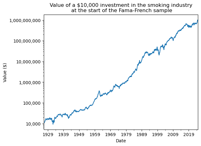
Artificial Intelligence (AI)
You may use AI (e.g., ChatGPT) to help you prepare your analysis and discussion. However:
- AI will not do very well on this project without significant input from your team
- AI will not be a defense against plagiarism because AI should not write your code and slides; If you plagiarize an AI that plagiarizes other sources, you are responsible for plagiarizing the AI and its sources
Function to Prepare Data File
Use this function to export your data file for the competition.
def write_csv(portfolio_returns, group_number):
    """
    Write portfolio returns to a CSV file named Group_XX.csv with Date as YYYY-MM.

    Parameters:
    - portfolio_returns: pandas Series or DataFrame with monthly returns (as decimals) and Date index
    - group_number: int, your two-digit group number (e.g., 1 for Group_01)

    Output:
    - Saves Group_XX.csv with two columns: Date (YYYY-MM) and Group_XX (returns as decimals)
    """

    # Make two-digit group number
    group_str = f"{group_number:02d}"
    filename = f"Group_{group_str}.csv"

    # Convert returns to DataFrame if Series
    if isinstance(portfolio_returns, pd.Series):
        df = portfolio_returns.to_frame(name=f"Group_{group_str}")
    else:
        df = portfolio_returns.rename(columns={portfolio_returns.columns[0]: f"Group_{group_str}"})

    # Convert index to PeriodIndex with monthly frequency and format as YYYY-MM
    if isinstance(df.index, pd.PeriodIndex):
        if df.index.freq != 'M':
            df.index = df.index.to_timestamp().to_period('M')
    elif isinstance(df.index, pd.DatetimeIndex):
        df.index = df.index.to_period('M')
    else:
        raise ValueError("Index must be a datetime or PeriodIndex")

    # Rename index to Date
    df.index.name = "Date"

    # Write to CSV
    df.to_csv(filename, index=True)

    print(f"Saved portfolio returns to {filename}")
# Example usage:
dates = pd.date_range(start="1931-07-01", end="1936-06-01", freq="MS")
returns = pd.Series([0.0025, 0.01, -0.005] + [0.001] * (len(dates) - 3), index=dates)
write_csv(returns, 1)Saved portfolio returns to Group_01.csvgroup_01 = (
pd.read_csv(
filepath_or_buffer='Group_01.csv',
parse_dates=['Date'],
na_values=[-99.99, -999]
)
.assign(Date=lambda x: x['Date'].dt.to_period('M'))
.set_index('Date')
.rename_axis(columns=['Team'])
.div(100)
)group_01.head()| Team | Group_01 |
|---|---|
| Date | |
| 1931-07 | 0.000025 |
| 1931-08 | 0.000100 |
| 1931-09 | -0.000050 |
| 1931-10 | 0.000010 |
| 1931-11 | 0.000010 |
Footnotes
To avoid this bias, I would give you anonymized data, you would automate your strategy into one function, and I would backtest your function output on a holdout sample. This process would be beyond the scope of this course.↩︎