import matplotlib.pyplot as plt
import numpy as np
import pandas as pd
import pandas_datareader as pdr
import seaborn as sns
from scipy.stats import norm # new addition for Monte Carlo methods
import warnings # to suppress the pandas_datareader warning
import yfinance as yfHerron Topic 5 - Practice - Sec 03
FINA 6333 for Spring 2025
%precision 2
pd.options.display.float_format = '{:.2f}'.format
# %config InlineBackend.figure_format = 'retina'
Announcements
- Programming assessment and MSFQ assessment will be in class and in person on Tuesday, 4/15, in your scheduled section
- Our plan for the rest of the semester
- Friday, 4/11, Project 2 solution, envelopes solution, and Project 3 group work
- Tuesday, 4/15, programming and MSFQ assessment in class and in person, in your scheduled section
- Friday, 4/18, Project 3 group work
- Tuesday, 4/22, Project 3 group work
- Wednesday, 4/23, Project 3 is due by 11:59 PM
- Friday, 4/25, office hours during regular class time
- Please complete TRACE! I value and use your feedback.
Five-Minute Recap
In finance, we use two main simulation methods: Monte Carlo and bootstrap. Both help analyze financial data, but work differently.
Monte Carlo methods create many possible paths of financial variables (e.g., stock prices, interest rates) based on theoretical probability distributions:
- Generates synthetic data from assumed models
- Creates data that may not exist in historical records
- Based on random sampling from probability distributions
- Think
np.random.uniform()ornp.random.normal()to create new random variables
Bootstrap methods take a different approach:
- Resamples from actual historical data (with or without replacement)
- Makes minimal assumptions about distributions
- Maintains statistical properties of original data
- Think
.sample()to resample past obervations
Practice
Estimate \(\pi\) by simulating darts thrown at a dart board
Hints: Select random \(x\)s and \(y\)s such that \(-r \leq x \leq +r\) and \(-r \leq x \leq +r\). Darts are on the board if \(x^2 + y^2 \leq r^2\). The area of the circlular board is \(\pi r^2\), and the area of square around the board is \((2r)^2 = 4r^2\). The fraction \(f\) of darts on the board is the same as the ratio of circle area to square area, so \(f = \frac{\pi r^2}{4 r^2}\).
First we throw darts at the board. Darts with \(x^2 + y^2 \leq r^2\) are on the board.
def throw_darts(n=1_000, r=1, seed=42):
    np.random.seed(seed)
    return (
        pd.DataFrame(
            data=np.random.uniform(low=-r, high=r, size=2*n).reshape(n, 2),
            columns=['X', 'Y']
        )
        .assign(On_Board=lambda x: x['X']**2 + x['Y']**2 <= r**2)
)throw_darts()| X | Y | On_Board | |
|---|---|---|---|
| 0 | -0.25 | 0.90 | True |
| 1 | 0.46 | 0.20 | True |
| 2 | -0.69 | -0.69 | True |
| 3 | -0.88 | 0.73 | False |
| 4 | 0.20 | 0.42 | True |
| ... | ... | ... | ... |
| 995 | 0.53 | -0.68 | True |
| 996 | 0.22 | -0.73 | True |
| 997 | 0.50 | 0.31 | True |
| 998 | 0.91 | -0.86 | False |
| 999 | -0.89 | -0.44 | True |
1000 rows × 3 columns
4 * throw_darts(n=1_000_000)['On_Board'].mean()3.14Next, we visualize these darts with a scatter plot. Seaborn’s scatterplot() helps color darts by location (i.e., on or off board). The .pipe() method lets us send the output of the .assign() method to sns.scatterplot() without assigning a temporary data frame.
(
    throw_darts(n=10_000)
    .assign(Location=lambda x: np.where(x['On_Board'], 'On Board', 'Off Board'))
    .pipe(
        sns.scatterplot,
        x='X',
        y='Y',
        hue='Location'
    )
)
plt.gca().set_aspect('equal')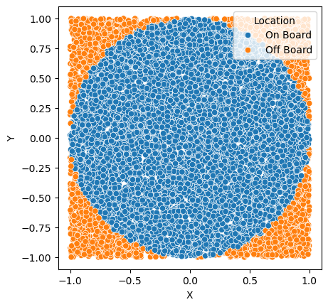
Finally, we use the hint above to estimate \(\pi\). The hint above says \(f = \frac{\pi r^2}{4 r^2}\), where \(f\) is the fraction of darts on the board. Therefore, \(\pi \approx \frac{4fr^2}{r^2} = 4f\). We increase the precision of our \(\pi\) estimate by increasing the number of simulated darts \(n\).
for n in 10**np.arange(7):
    print(f'With {n:>9,.0f} dart throws, our estimate of pi is: {4 * throw_darts(n=n)['On_Board'].mean():,.4f}')
With 1 dart throws, our estimate of pi is: 4.0000
With 10 dart throws, our estimate of pi is: 3.2000
With 100 dart throws, our estimate of pi is: 3.0400
With 1,000 dart throws, our estimate of pi is: 3.1040
With 10,000 dart throws, our estimate of pi is: 3.1544
With 100,000 dart throws, our estimate of pi is: 3.1468
With 1,000,000 dart throws, our estimate of pi is: 3.1420Simulate your wealth \(W_T\) by randomly sampling market returns
Use monthly market returns from the French Data Library. Only invest one cash flow \(W_0\), and plot the distribution of \(W_T\).
First, we download data from the French Data Library. We convert these returns from percent to decimal to simplify compounding.
with warnings.catch_warnings():
    warnings.filterwarnings("ignore", category=FutureWarning)
    ff3 = (
        pdr.DataReader(
            name='F-F_Research_Data_Factors',
            data_source='famafrench',
            start='1900'
        )
        [0]
        .assign(Mkt=lambda x: x['Mkt-RF'] + x['RF'])
        .div(100)
)- Use
.sample()to simulate one alternate history - Add
pd.concat()and a list comprehension to simulateNalternate histories - Examine/plot the distributoin of
W_T
ff3['Mkt'].sample(n=5, random_state=42, ignore_index=True)0 0.03
1 0.03
2 0.04
3 -0.11
4 -0.02
Name: Mkt, dtype: float64We can combine many samples of many months with a list comprehension and pd.concat().
W_0 = 50_000
T = 30 * 12
N = 1_000

r_t = pd.concat(
    objs=[ff3['Mkt'].sample(n=T, random_state=i, ignore_index=True) for i in range(N)],
    keys=range(N),
    names=['Simulation'],
    axis=1
)r_t.iloc[:5, :5]| Simulation | 0 | 1 | 2 | 3 | 4 |
|---|---|---|---|---|---|
| 0 | 0.04 | 0.01 | 0.02 | 0.03 | 0.08 |
| 1 | -0.03 | -0.02 | 0.04 | 0.01 | -0.02 |
| 2 | -0.00 | 0.06 | 0.06 | 0.02 | 0.00 |
| 3 | -0.05 | -0.02 | 0.04 | 0.02 | -0.05 |
| 4 | 0.02 | -0.04 | -0.01 | -0.02 | 0.00 |
W_T = W_0 * r_t.add(1).prod()We visualize terminal wealth \(W_T\) with a cumulative distribution plot.
W_T.plot(kind='hist', cumulative=True, density=True, bins=100, logx=True)
plt.xlabel('Terminal Wealth ($)')
plt.title(f'Terminal Wealth of ${W_0:,.0f} Initial Investment\n for {N} Simulations of {T} Months')
plt.show()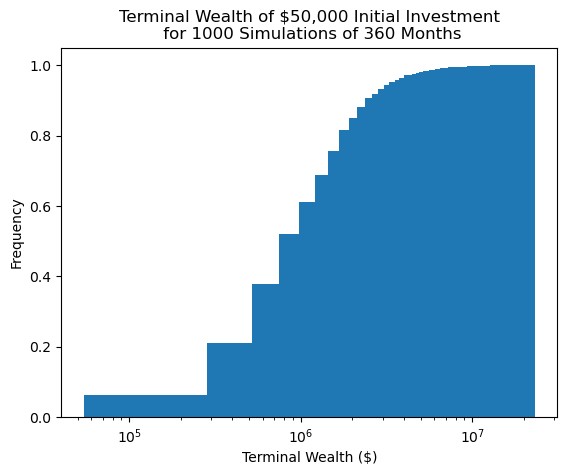
The plot above may be difficult to read and interpret because \(W_T\) has large outliers. We can use a for to calculate several levels of confidence.
for i in [0.01, 0.02, 0.03, 0.04, 0.05]:
    print(f'In {100-100*i:,.0f}% of outcomes, an initial investment of ${W_0:,.0f} for {T} months has a terminal wealth greater than ${W_T.quantile(i):,.0f}')
In 99% of outcomes, an initial investment of $50,000 for 360 months has a terminal wealth greater than $146,041
In 98% of outcomes, an initial investment of $50,000 for 360 months has a terminal wealth greater than $195,993
In 97% of outcomes, an initial investment of $50,000 for 360 months has a terminal wealth greater than $215,765
In 96% of outcomes, an initial investment of $50,000 for 360 months has a terminal wealth greater than $240,818
In 95% of outcomes, an initial investment of $50,000 for 360 months has a terminal wealth greater than $271,537Repeat the exercise above but add end-of-month investments \(C_t\)
We can use the same data frame r_t of simulated market returns. However, need to consider end-of-month investments of C_t. The easiest approach is to write a for that starts with W_last = W_0, then each month updates W_last = W_last * (1 + r) + C_t. Finally, it pd.concat()s these monthly values of W_last into a data frame of monthly wealths W_t.
C_t = 1_000
W_last = W_0
W_t = []

for i, r in r_t.iterrows():
    W_last = (1 + r) * W_last + C_t
    W_t.append(W_last)

W_t = pd.concat(objs=W_t, axis=1, keys=r_t.index).transpose()W_t.iloc[:5, :5]| Simulation | 0 | 1 | 2 | 3 | 4 |
|---|---|---|---|---|---|
| 0 | 53190.00 | 51595.00 | 51805.00 | 52455.00 | 54830.00 |
| 1 | 52860.25 | 51449.59 | 54726.97 | 54178.88 | 54996.58 |
| 2 | 53743.96 | 55613.74 | 58829.98 | 56051.16 | 56106.58 |
| 3 | 52051.39 | 55662.75 | 62400.85 | 57919.95 | 54318.08 |
| 4 | 54087.21 | 54514.16 | 62864.21 | 57645.71 | 55328.94 |
W_T = W_t.iloc[-1]W_T.plot(kind='hist', cumulative=True, density=True, bins=100, logx=True)
plt.xlabel('Terminal Wealth ($)')
plt.title(f'Terminal Wealth of ${W_0:,.0f} Initial Investment\n for {N} Simulations of {T} Months with ${C_t} Investments')
plt.show()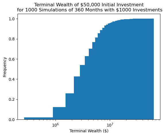
for i in [0.01, 0.02, 0.03, 0.04, 0.05]:
    print(f'In {100-100*i:,.0f}% of outcomes, an initial investment of ${W_0:,.0f} for {T} months with ${C_t} investments has a terminal wealth greater than ${W_T.quantile(i):,.0f}')
In 99% of outcomes, an initial investment of $50,000 for 360 months with $1000 investments has a terminal wealth greater than $786,650
In 98% of outcomes, an initial investment of $50,000 for 360 months with $1000 investments has a terminal wealth greater than $900,482
In 97% of outcomes, an initial investment of $50,000 for 360 months with $1000 investments has a terminal wealth greater than $996,068
In 96% of outcomes, an initial investment of $50,000 for 360 months with $1000 investments has a terminal wealth greater than $1,094,423
In 95% of outcomes, an initial investment of $50,000 for 360 months with $1000 investments has a terminal wealth greater than $1,167,491