import matplotlib.pyplot as plt
import numpy as np
import pandas as pd
import pandas_datareader as pdr
import yfinance as yfHerron Topic 1 - Log and Simple Returns, Portfolio Math, and Applications - Blank
FINA 6333 for Spring 2025
This notebook covers two topics:
- Log and simple returns
- Portfolio returns, plus two applications of portfolio returns
%precision 4
pd.options.display.float_format = '{:.4f}'.format
# %config InlineBackend.figure_format = 'retina'
Log and Simple Returns
We will typically use simple returns, calculated as \(r_{simple,t} = \frac{p_t + d_t - p_{t-1}}{p_{t-1}}\). This simple return is the return that investors earn on their investments. We can calculate simple returns from Yahoo Finance data with the .pct_change() method on the adjusted close column (i.e., Adj Close), which adjusts for dividends and splits. The adjusted close column is a reverse-engineered close price (i.e., end-of-trading-day price) that incorporates dividends and splits, making simple return calculations easy.
However, we may see log returns elsewhere, which are the (natural) log of one plus simple returns: \(r_{log,t} = \log(1 + r_{simple,t})\). Therefore, we calculate log returns as either the log of one plus simple returns or the difference of the logs of the adjusted close column. Log returns are also known as continuously-compounded returns.
This section explains the differences between simple and log returns and where each is appropriate.
Simple and Log Returns are Similar for Small Returns
\(x \approx \log(1 + x)\) for small values of \(x\), so simple returns and log returns are similar for small returns. Returns are typically small at daily and monthly horizons, so the difference between simple and log returns is small at daily and monthly horizons. The following figure shows that \(r_{simple,t} \approx r_{log,t}\) for small values of \(r\).
simpler = np.linspace(-0.75, 0.75, 100)
logr = np.log1p(simpler)
plt.plot(simpler, logr)
plt.plot([-1, 1], [-1, 1])
plt.xlabel('Simple Return')
plt.ylabel('Log Return')
plt.title('Log Versus Simple Returns')
plt.legend(['Actual Relation', 'Relation If Log = Simple'])
plt.show()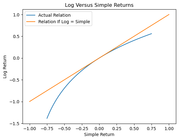
Simple Return Advantage: Portfolio Calculations
For a portfolio of \(N\) assets with portfolio weights \(w_i\), the portfolio return \(r_p\) is the weighted average of the returns of its assets: \(r_p = \sum_{i=1}^N w_i r_{i}\). For example, for an equal-weighted portfolio with two stocks, \(r_p = 0.5 r_1 + 0.5 r_2 = \frac{r_1 + r_2}{2}\). Therefore, we cannot calculate portfolio returns with log returns because the sum of logs is the log of products. That is \(\log(1+r_i) + \log(1+r_j) = \log((1+r_i) \times (1+r_j))\), which is not what we want to measure! We cannot perform portfolio calculations with log returns!
Log Return Advantage: Log Returns are Additive
We compound simple returns with multiplication, but we compound log returns with addition. This additive property of log returns makes code simple, computations fast, and proofs easy when we must compound returns.
We compound returns from \(t=0\) to \(t=T\) as follows: \[1 + r_{0, T} = (1 + r_1) \times (1 + r_2) \times \dots \times (1 + r_T)\] Next, we take the log of both sides of the previous equation and use the property that the log of products is the sum of logs: \[\log(1 + r_{0, T}) = \log((1 + r_1) \times (1 + r_2) \times \dots \times (1 + r_T)) = \log(1 + r_1) + \log(1 + r_2) + \dots + \log(1 + r_T) = \sum_{t=1}^T \log(1 + r_t)\] Next, we exponentiate both sides of the previous equation: \[e^{\log(1 + r_{0, T})} = e^{\sum_{t=0}^T \log(1 + r_t)}\] Next, we use the property that \(e^{\log(x)} = x\) to simplify the previous equation: \[1 + r_{0,T} = e^{\sum_{t=0}^T \log(1 + r_t)}\] Finally, we subtract 1 from both sides: \[r_{0 ,T} = e^{\sum_{t=0}^T \log(1 + r_t)} - 1\] So, the return \(r_{0,T}\) from \(t=0\) to \(t=T\) is the exponentiated sum of log returns. The pandas developers assume users understand the math above and focus on optimizing sums!
np.random.seed(42)
df = pd.DataFrame(data={'r': np.exp(np.random.randn(10_000)) - 1})

df.describe()| r | |
|---|---|
| count | 10000.0000 |
| mean | 0.6529 |
| std | 2.1918 |
| min | -0.9802 |
| 25% | -0.4896 |
| 50% | -0.0026 |
| 75% | 0.9564 |
| max | 49.7158 |
We can time the calculation of 10-observation rolling returns. We use .apply() for the simple return version because .rolling() does not have a product method. We find that .rolling() is slower with .apply() than with .sum() by a factor of about 1,000. We will learn about .rolling() and .apply() in a few weeks, but they provide the best example of when to use log returns.
%%timeit
df['r10_via_prod'] = (
    df['r']
    .add(1)
    .rolling(10)
    .apply(lambda x: x.prod())
    .sub(1)
)
936 ms ± 119 ms per loop (mean ± std. dev. of 7 runs, 10 loops each)%%timeit
df['r10_via_sum'] = (
df['r']
.add(1)
.pipe(np.log)
.rolling(10)
.sum()
.pipe(np.exp)
.sub(1)
)1.15 ms ± 159 μs per loop (mean ± std. dev. of 7 runs, 1,000 loops each)df.head(15)| r | r10_via_prod | r10_via_sum | |
|---|---|---|---|
| 0 | 0.6433 | NaN | NaN |
| 1 | -0.1291 | NaN | NaN |
| 2 | 0.9111 | NaN | NaN |
| 3 | 3.5861 | NaN | NaN |
| 4 | -0.2088 | NaN | NaN |
| 5 | -0.2087 | NaN | NaN |
| 6 | 3.8511 | NaN | NaN |
| 7 | 1.1542 | NaN | NaN |
| 8 | -0.3747 | NaN | NaN |
| 9 | 0.7204 | 87.2886 | 87.2886 |
| 10 | -0.3709 | 32.8006 | 32.8006 |
| 11 | -0.3723 | 23.3617 | 23.3617 |
| 12 | 0.2737 | 15.2369 | 15.2369 |
| 13 | -0.8524 | -0.4774 | -0.4774 |
| 14 | -0.8218 | -0.8823 | -0.8823 |
np.allclose(df['r10_via_prod'], df['r10_via_sum'], equal_nan=True)TrueThese two approaches calculate the same return series, but the simple-return approach using .prod() is about 1,000 times slower than the log-return approach using .sum()! We can use log returns to calculate total returns very quickly!
Portfolio Math
Portfolio return \(r_{p}\) is the weighted average of its asset returns, so \(r_{p} = \sum_{i=1}^N w_i r_{i}\). Here \(N\) is the number of assets, \(w_i\) is the weight on asset \(i\), and \(\sum_{i=1}^N w_i = 1\).
The 1/N Portfolio
The \(\frac{1}{N}\) portfolio equally weights portfolio assets, so \(w_1 = w_2 = \dots = w_N = \frac{1}{N}\). If \(w_i = \frac{1}{N}\), then \(r_{p} = \sum_{i=1}^N \frac{1}{N} r_{i} = \frac{\sum_{i=1}^N r_i}{N} = \bar{r}\). Therefore, we can use .mean(axis=1) to calculate \(\frac{1}{N}\) portfolio returns!
df2 = yf.download(tickers='AAPL AMZN GOOG MSFT NVDA TSLA', auto_adjust=False, progress=False).iloc[:-1]
returns2 = df2['Adj Close'].pct_change().dropna()

returns2.describe()| Ticker | AAPL | AMZN | GOOG | MSFT | NVDA | TSLA |
|---|---|---|---|---|---|---|
| count | 3689.0000 | 3689.0000 | 3689.0000 | 3689.0000 | 3689.0000 | 3689.0000 |
| mean | 0.0011 | 0.0012 | 0.0009 | 0.0010 | 0.0021 | 0.0021 |
| std | 0.0175 | 0.0205 | 0.0173 | 0.0161 | 0.0288 | 0.0362 |
| min | -0.1286 | -0.1405 | -0.1110 | -0.1474 | -0.1876 | -0.2106 |
| 25% | -0.0074 | -0.0089 | -0.0071 | -0.0070 | -0.0122 | -0.0164 |
| 50% | 0.0010 | 0.0010 | 0.0009 | 0.0007 | 0.0017 | 0.0012 |
| 75% | 0.0102 | 0.0119 | 0.0093 | 0.0093 | 0.0161 | 0.0194 |
| max | 0.1198 | 0.1575 | 0.1605 | 0.1422 | 0.2981 | 0.2440 |
returns2.mean() # implied axis=0Ticker
AAPL 0.0011
AMZN 0.0012
GOOG 0.0009
MSFT 0.0010
NVDA 0.0021
TSLA 0.0021
dtype: float64rp2_via_mean = returns2.mean(axis=1)
rp2_via_meanDate
2010-06-30 -0.0123
2010-07-01 -0.0107
2010-07-02 -0.0271
2010-07-06 -0.0223
2010-07-07 0.0254
...
2025-02-21 -0.0272
2025-02-24 -0.0127
2025-02-25 -0.0247
2025-02-26 -0.0055
2025-02-27 -0.0330
Length: 3689, dtype: float64Note that when we apply the same portfolio weights every period, we rebalance at the same frequency as the returns data. If we have daily data, rebalance daily. If we have monthly data, we rebalance monthly, and so on.
A More General Solution
If we combine portfolio weights into vector \(w\) and the time series of asset returns into matrix \(\mathbf{R}\), then we can calculate the time series of portfolio returns as \(r_p = w^T \mathbf{R}\). The pandas version of this calculation is R.dot(w), where R is a data frame of asset returns and w is a series or an array of portfolio weights. We can use this approach to calculate \(\frac{1}{N}\) portfolio returns, too.
weights2 = np.ones(returns2.shape[1]) / returns2.shape[1]

weights2
array([0.1667, 0.1667, 0.1667, 0.1667, 0.1667, 0.1667])rp2_via_dot = returns2.dot(weights2)
rp2_via_dotDate
2010-06-30 -0.0123
2010-07-01 -0.0107
2010-07-02 -0.0271
2010-07-06 -0.0223
2010-07-07 0.0254
...
2025-02-21 -0.0272
2025-02-24 -0.0127
2025-02-25 -0.0247
2025-02-26 -0.0055
2025-02-27 -0.0330
Length: 3689, dtype: float64Both approaches give the same answer!
np.allclose(rp2_via_mean, rp2_via_dot, equal_nan=True)TruePortfolio Math Application 1: All stocks half the time or half stocks all the time?
Are you better off investing:
- 100% in stocks 50% of the time and the riskless asset the other 50% of the time or
- 50% in stocks and 50% in the riskless asset 100% of the time?
Here is a roadmap for convincing yourself with data!
Download annual market and risk-free asset returns from Kenneth French’s data library
Convert these factors to decimal returns and calculate the market return series
Add a portfolio return series that is half stocks all the time
You might call this portfolio return series Balanced
Add a portfolio return series that switches between stocks and bills every year with stocks in odd years
You might call this portfolio return series Switching Stocks Odd
Add a portfolio return series that switches between stocks and bills every year with stocks in even years
You might call this portfolio return series Switching Stocks Even
Plot the cumulative returns calculate the summary statistics for the Balanced and Switching series
Use the .describe() method to calcualte summary statistics.
Which strategy do you prefer?
Why? How sure are you?
Use the simulate() function to simulate 10,000 different outcomes for the U.S. market
simulate() calculates one Switching return series because the randomization also randomizes the odd-year and even-year choice.
def simulate(df, cols=['Mkt', 'RF'], n_iter=10_000):
    """
    Simulates resampling of the given DataFrame columns and computes bal;anced and switching portfolio returns.

    Parameters:
    df (pd.DataFrame): The input DataFrame.
    cols (list): List of column names to sample.
    n_iter (int): Number of iterations for simulation.

    Returns:
    pd.DataFrame: A concatenated DataFrame with simulation results.
    """
    return pd.concat(
        objs=[(
            df[cols]
            .sample(frac=1, ignore_index=True, random_state=i)
            .assign(
                Balanced=lambda x: x[cols].mean(axis=1),
                Switching=lambda x: np.where(x.index % 2 == 0, x[cols[0]], x[cols[1]])
            )
        ) for i in range(n_iter)],
        keys=range(n_iter),
        names=['Simulation', 'Year']
    )
Calculate the summary statistics for these new Balanced and Switching series
Which strategy do you prefer?
Why? How sure are you?
Portfolio Math Application 2: What are the benefits of diversification?
Use random portfolios of S&P 100 stocks of various portfolio sizes to show that portfolio volatility falls quickly, then slowly, then not at all as we increase portfolio size.
Download daily data for the stocks in the S&P 100
Wikipedia provides tickers for the stocks in the S&P 100. Use a list comprehension to replace . in tickers with - for compatability with Yahoo! Finance.
Calculate the past five years of dailty returns for these stocks
Calculate the volatilies of 20 equal-weighted random portfolios of various portfolio sizes
Random portfolios should have portfolio sizes of 1, 2, 4, 6, 8, 10, 20, 30, 40, or 50 stocks each.
You can combine the .sample(n=?, axis=1, random_state=?), .mean(axis=1), and .std() to calculate the volatilities of equal-weighted portfolios. You can collect these volatilies in a list of lists built with two for loops or list comprehensions. Replace the ?s in .sample() with loop counters. The inner loop will calculate a portfolio volatilty for each portfolio size, and the outer loop will collect 20 versions of each portfolio. Using the outer loop counter for random_state= makes your analysis repeatable!