import matplotlib.pyplot as plt
import numpy as np
import pandas as pd
import pandas_datareader as pdr
import scipy.optimize as sco # new addition for portfolio optimization
import statsmodels.api as sm
import yfinance as yfHerron Topic 4 - Portfolio Optimization
FINA 6333 for Spring 2025
%precision 4
pd.options.display.float_format = '{:.4f}'.format
# %config InlineBackend.figure_format = 'retina'
Introduction
This notebook covers portfolio optimization. In this notebook, we will:
- Review the 1/N portfolio (or equal-weighted portfolio) from the Herron topic 1 notebook
- Use SciPy’s
minimize()function to:- Find the minimum-variance portfolio
- Find the minimum-variance frontier
Ivo Welch provides a clear discussion of the theory and practice of portfolio optimization in Chapter 12 of his free investments textbook.
The 1/N Portfolio
We first saw the 1/N portfolio (or equal-weighted portfolio) in the Herron topic 1 notebook. The 1/N portfolio gives each of N assets an equal portfolio weight of 1/N. While the 1/N strategy seems too simple to be useful, DeMiguel, Garlappi, and Uppal (2009) show the 1/N portfolio typically has a higher mean-variance efficiency than advanced portfolio optimizations.
We will investigate the 1/N portfolio and portfolio optimization with the most recent three years of daily returns for the Mag 7 stocks (i.e., GOOGL, AMZN, AAPL, META, MSFT, NVDA, and TSLA).
mag7 = (
    yf.download(
        tickers='GOOGL AMZN AAPL META MSFT NVDA TSLA',
        auto_adjust=False,
        progress=False
    )
    .iloc[:-1] # drop incomplete trading day
)
returns = (
mag7
['Adj Close']
.pct_change()
.iloc[(-3 * 252):]
)We can manually calculate 1/N portfolio returns three ways.
The first calculation is a literal interpretation of \(r_P = \frac{1}{N} \sum_{i}^{N} r_i\). The pandas code for this first calculation is returns.sum(axis=1).div(n), which sums across the rows, and then divides by n. Recall that with constant weights, we rebalance our portfolio every return period. If we have daily data, we rebalance daily. If we have monthly data, we rebalance monthly, and so on.
n = returns.shape[1]
r_p1 = returns.sum(axis=1).div(n)r_p1.describe()count 756.0000
mean 0.0010
std 0.0196
min -0.0674
25% -0.0099
50% 0.0007
75% 0.0127
max 0.0984
dtype: float64We learned the last two calculations in the Herron topic 1. The pandas code for the second calculation is returns.mean(axis=1), which calculates the mean of each row.
r_p2 = returns.mean(axis=1)r_p2.describe()count 756.0000
mean 0.0010
std 0.0196
min -0.0674
25% -0.0099
50% 0.0007
75% 0.0127
max 0.0984
dtype: float64The pandas code for the third calculations is returns.dot(weights), where weights is a NumPy array or a pandas series of portfolio weights. This calculation allows different weights for each asset. We can make 1/N portfolio weights with np.ones(n) / n.
weights = np.ones(n) / nweightsarray([0.1429, 0.1429, 0.1429, 0.1429, 0.1429, 0.1429, 0.1429])r_p3 = returns.dot(weights)r_p3.describe()count 756.0000
mean 0.0010
std 0.0196
min -0.0674
25% -0.0099
50% 0.0007
75% 0.0127
max 0.0984
dtype: float64We can use np.allclose() to show that r_p1, r_p2, and r_p3 are similar.
np.allclose(r_p1, r_p2)Truenp.allclose(r_p2, r_p3)Truenp.allclose(r_p3, r_p1)TrueHere is a brief detour to show how the .dot() method works.
silly_n = 3
silly_w = np.ones(silly_n) / silly_n
silly_r = pd.DataFrame(np.arange(2*silly_n).reshape(2, silly_n))print(
f'silly_n:\n{silly_n}',
f'silly_w:\n{silly_w}',
f'silly_r:\n{silly_r}',
sep='\n\n'
)silly_n:
3
silly_w:
[0.3333 0.3333 0.3333]
silly_r:
0 1 2
0 0 1 2
1 3 4 5silly_r.dot(silly_w)0 1.0000
1 4.0000
dtype: float64Under the hood, the .dot() method efficiently calculates the following:
for i, row in silly_r.iterrows():
    print(
        f'Row {i}: ',
        ' + '.join([f'{w:0.2f} * {y}' for w, y in zip(silly_w, row)]),
        ' = ',
        f'{silly_r.dot(silly_w).iloc[i]:0.2f}'
    )
Row 0: 0.33 * 0 + 0.33 * 1 + 0.33 * 2 = 1.00
Row 1: 0.33 * 3 + 0.33 * 4 + 0.33 * 5 = 4.00SciPy’s minimize() Function
SciPy’s minimize() function, from the optimize module, finds the input array x that minimizes the output of a given function fun. The minimize() function uses optimization techniques that are beyond the scope of this course. We can consider these optimization techniques as sophisticated trial-and-error (or guess-and-check).
Here are the common arguments for the the minimize() function:
fun=is the name of the function who’s output we want to minimizex0=is our first guess for the input to the functionfunargs=is a tuple of additional arguments to the functionfunbounds=is a tuple of tuples with lower and upper bounds for each element inxcontraints=is a tuple of dictionaries that limitxby constraining the output of a given function to zero or non-negative values
Here is a simple example that minimizes the function quadratic(), which has arguments \(x\) and \(a\) and returns \((x - a)^2\).
def quadratic(x, a=5):
return (x - a) ** 2quadratic(x=0, a=5)25quadratic(x=5, a=5)0quadratic(x=10, a=5)25It might be helpful to plot \(y = (x - a)^2\).
x = np.linspace(-5, 15, 101)
y = quadratic(x=x)
plt.plot(x, y)
plt.xlabel(r'$x$')
plt.ylabel(r'$y$')
plt.title(r'$y = (x - 5)^2$ over $x \in [-5, 15]$')
plt.show()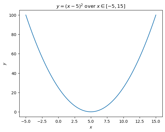
The minimum output of quadratic() occurs at \(x=5\) if we do not use bounds or constraints. For this function, we can even start far away from \(x=5\).
sco.minimize(
    fun=quadratic,
    x0=np.array([2001])
)
message: Optimization terminated successfully.
success: True
status: 0
fun: 2.0392713450495178e-16
x: [ 5.000e+00]
nit: 4
jac: [-1.366e-08]
hess_inv: [[ 5.000e-01]]
nfev: 18
njev: 9The minimum output of quadratic() occurs at \(x=6\) if we bound \(6 \leq x \leq 10\) with bounds=((6, 10),). bounds= requires a tuple of tuples, so we need the trailing comma if we only have one set of bounds.
sco.minimize(
    fun=quadratic,
    x0=np.array([2001]),
    bounds=((6, 10),)
)
message: CONVERGENCE: NORM OF PROJECTED GRADIENT <= PGTOL
success: True
status: 0
fun: 1.0
x: [ 6.000e+00]
nit: 1
jac: [ 2.000e+00]
nfev: 4
njev: 2
hess_inv: <1x1 LbfgsInvHessProduct with dtype=float64>The minimum output of quadratic() also occurs at \(x=6\) if we constrain \(x-6 \geq 0\) with constraints=({'type': 'ineq', 'fun': lambda x: x - 6}). For inequality constraints, the given function must evaluate to a non-negative value. We use bounds to limit the search space directly, and we use constraints to limit the search space based on a given function.
sco.minimize(
    fun=quadratic,
    x0=np.array([2001]),
    constraints=({'type': 'ineq', 'fun': lambda x: x - 6})
)
message: Optimization terminated successfully
success: True
status: 0
fun: 1.0000000000000018
x: [ 6.000e+00]
nit: 3
jac: [ 2.000e+00]
nfev: 6
njev: 3We use the args= argument to pass additional arguments to the function fun. For example, we change the a= argument in quadratic() from the default of a=5 to a=20 with args=(20,). Like bounds=, args= expects a tuple, so we need a trailing comma if we have only one argument.
sco.minimize(
    fun=quadratic,
    args=(20,),
    x0=np.array([2001]),
)
message: Optimization terminated successfully.
success: True
status: 0
fun: 7.090392030754976e-17
x: [ 2.000e+01]
nit: 4
jac: [-1.940e-09]
hess_inv: [[ 5.000e-01]]
nfev: 18
njev: 9The Minimum-Variance Portfolio
Now we apply minimize() to our Mag-7 returns to find the the minimum-variance portfolio. Recall, the minimize() function varies an input array x, starting from argument x0=, to minimize the output of a given function fun= subject to the bounds and constraints in bounds= and constraints=, respectively.
We can define a function calc_sigmap() to calculate portfolio volatility. The first argument to calc_sigmap() must be the input array x that minimize() searches over. We call this first argument w because it has portfolio weights. Recall that portfolio variance is \(\sigma^2_p = w' \Sigma w\), so portfolio volatility is \(\sigma_p = \sqrt{w' \Sigma w}\). Here \(\Sigma\) (and Sigma) is the returns covariance matrix, and \(w\) (and w) is the portfolio weights array.
def calc_sigmap(w, Sigma, ppy=252):
    return np.sqrt(ppy * w.T @ Sigma @ w)
Sigma = returns.cov()Sigma| Ticker | AAPL | AMZN | GOOGL | META | MSFT | NVDA | TSLA |
|---|---|---|---|---|---|---|---|
| Ticker | |||||||
| AAPL | 0.0003 | 0.0002 | 0.0002 | 0.0002 | 0.0002 | 0.0003 | 0.0003 |
| AMZN | 0.0002 | 0.0005 | 0.0003 | 0.0004 | 0.0003 | 0.0004 | 0.0004 |
| GOOGL | 0.0002 | 0.0003 | 0.0004 | 0.0003 | 0.0002 | 0.0004 | 0.0003 |
| META | 0.0002 | 0.0004 | 0.0003 | 0.0008 | 0.0003 | 0.0005 | 0.0004 |
| MSFT | 0.0002 | 0.0003 | 0.0002 | 0.0003 | 0.0003 | 0.0004 | 0.0003 |
| NVDA | 0.0003 | 0.0004 | 0.0004 | 0.0005 | 0.0004 | 0.0012 | 0.0006 |
| TSLA | 0.0003 | 0.0004 | 0.0003 | 0.0004 | 0.0003 | 0.0006 | 0.0015 |
We can also define a function calc_mup() that calculates a mean portfolio return. Recall that mean portfolio return is \(\mu_p = w' \mu\). Here \(\mu\) (and mu) is the mean returns array, and \(w\) (and w) is the portfolio weights array.
def calc_mup(w, mu, ppy=252):
    return ppy * w.T @ mu
mu = returns.mean()muTicker
AAPL 0.0005
AMZN 0.0005
GOOGL 0.0004
META 0.0018
MSFT 0.0005
NVDA 0.0025
TSLA 0.0005
dtype: float64Finally, we can use minimize() to find the portfolio weights that minimize portfolio volatility. Below, the equality constraint is met when x.sum() - 1 is zero, which is the Python equivalent of \(\sum_i w_i = 1\).
[(0,1) for _ in Sigma][(0, 1), (0, 1), (0, 1), (0, 1), (0, 1), (0, 1), (0, 1)]res_mv = sco.minimize(
fun=calc_sigmap,
x0=np.ones(Sigma.shape[0]) / Sigma.shape[0],
args=(Sigma, 252),
bounds=[(0,1) for _ in Sigma],
constraints=(
{'type': 'eq', 'fun': lambda x: x.sum() - 1},
)
)print(res_mv) message: Optimization terminated successfully
success: True
status: 0
fun: 0.2434752847371044
x: [ 4.614e-01 0.000e+00 9.627e-02 2.819e-18 4.423e-01
4.207e-17 9.975e-18]
nit: 10
jac: [ 2.435e-01 2.573e-01 2.435e-01 2.770e-01 2.435e-01
3.424e-01 3.046e-01]
nfev: 80
njev: 10What are the attributes of the minimum-variance portfolio? We can write a helper function print_port_res() to simplify our lives!
def print_port_res(w, mu, Sigma, title, ppy=252):
    width = max(len(title), 32)
    mup = ppy * w.T @ mu
    sigmap = np.sqrt(ppy * w.T @ Sigma @ w)

    return print(
        title,
        '=' * width,
        '',
        'Performance',
        '-' * width,
        'Annualized Mean Return:'.ljust(width - 6) + f'{mup:0.4f}',
        'Annualized Volatility:'.ljust(width - 6) + f'{sigmap:0.4f}',
        '',
        'Weights',
        '-' * width,
        '\n'.join([
            f'{_r}:'.ljust(width - 6) + f'{_w:0.4f}'
            for _r, _w in zip(Sigma.index, w)
        ]),
        '=' * width,
        sep='\n',
    )
print_port_res(
w=res_mv['x'],
mu=returns.mean(),
Sigma=returns.cov(),
title='minimum-variance portfolio'
)minimum-variance portfolio
================================
Performance
--------------------------------
Annualized Mean Return: 0.1292
Annualized Volatility: 0.2435
Weights
--------------------------------
AAPL: 0.4614
AMZN: 0.0000
GOOGL: 0.0963
META: 0.0000
MSFT: 0.4423
NVDA: 0.0000
TSLA: 0.0000
================================The Minimum-Variance Frontier
We can use minimize() to find the minimum-variance portfolio for a target return, then use a for loop to repeat this calculation for a wide range of target returns. This calculation will map out the minimum-variance frontier. Here are the steps:
- Create a NumPy array
returns_targetof target returns - Create an empty list
res_efto holdminimize()results - Loop over
returns_target, passing each target return as a constraint tominimize() - Append each
minimize()result tores_ef
returns_target = 252 * np.linspace(
    start=mu.min(),
    stop=mu.max(),
    num=50
)returns_target[:5]array([0.1035, 0.1143, 0.1251, 0.1359, 0.1467])Below, the first equality constraint is met when x.sum() - 1 is zero, which is the Python equivalent of \(\sum_i w_i = 1\). The second equality constraint is met when calc_mup(w=x, mu=mu, ppy=252) - r is zero, which is the Python equivbalent of \(w' \mu = \text{target return}\).
res_ef = []

for r in returns_target:
    _ = sco.minimize(
        fun=calc_sigmap,
        x0=np.ones(Sigma.shape[0]) / Sigma.shape[0],
        args=(Sigma, 252),
        bounds=[(0, 1) for c in Sigma.index],
        constraints=(
            {'type': 'eq', 'fun': lambda x: x.sum() - 1},
            {'type': 'eq', 'fun': lambda x: calc_mup(w=x, mu=mu, ppy=252) - r}
        )
    )
    res_ef.append(_)
The list res_ef contains the results of all 50 minimum-variance portfolios. For example, res_ef[0] is the minimum-variance portfolio for the lowest target return.
res_ef[0] message: Optimization terminated successfully
success: True
status: 0
fun: 0.3237995797768805
x: [ 0.000e+00 1.110e-16 1.000e+00 2.776e-16 5.171e-08
0.000e+00 0.000e+00]
nit: 2
jac: [ 1.592e-01 2.418e-01 3.238e-01 2.692e-01 1.773e-01
2.893e-01 2.533e-01]
nfev: 16
njev: 2print_port_res(
w=res_ef[0]['x'],
mu=mu,
Sigma=Sigma,
title='minimum-variance portfolio for lowest tgt. ret.'
)minimum-variance portfolio for lowest tgt. ret.
===============================================
Performance
-----------------------------------------------
Annualized Mean Return: 0.1035
Annualized Volatility: 0.3238
Weights
-----------------------------------------------
AAPL: 0.0000
AMZN: 0.0000
GOOGL: 1.0000
META: 0.0000
MSFT: 0.0000
NVDA: 0.0000
TSLA: 0.0000
===============================================We should check that all minimizations suceeded. If a portfolio volatility minimization fails, we should check our function, bounds, and constraints. Portfolio optimization is typically a simple problem for minimize(), so we typically have an error if minimize() does not succeed.
for r in res_ef:
    assert r['success']
We can combine the target returns and volatilities into a data frame mv_frontier.
mv_frontier = pd.DataFrame({
    'returns_target': returns_target,
    'volatility': np.array([r['fun'] if r['success'] else np.nan for r in res_ef])
})
Finally, we can plot the minimum-variance frontier.
(
    mv_frontier
    .mul(100)
    .plot(x='volatility', y='returns_target', legend=False)
)
plt.ylabel('Annualized Mean Return (%)')
plt.xlabel('Annualized Volatility (%)')

for t in Sigma.index:
    x = 100 * np.sqrt(252 * Sigma.loc[t, t])
    y = 100 * 252 * mu.loc[t]
    plt.annotate(text=t, xy=(x, y))

plt.show()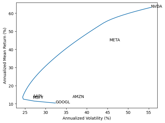
References
DeMiguel, Victor, Lorenzo Garlappi, and Raman Uppal. 2009. “Optimal Versus Naive Diversification: How Inefficient Is the 1/n Portfolio Strategy?” The Review of Financial Studies 22 (5): 1915–53.