import matplotlib.pyplot as plt
import numpy as np
import pandas as pd
import pandas_datareader as pdr
import scipy.optimize as sco # new addition for portfolio optimization
import statsmodels.api as sm
import yfinance as yfHerron Topic 4 - Practice - Sec 02
FINA 6333 for Spring 2025
%precision 4
pd.options.display.float_format = '{:.4f}'.format
# %config InlineBackend.figure_format = 'retina'
Announcements
- Please complete TRACE! I use TRACE to improve my treaching and courses, and I value your feedback. More here: https://northeastern.instructure.com/courses/207607/discussion_topics/2753925
- Please plan for the in-class programming and MSFQ assessments on Tuesday, 4/15
Five-Minute Recap
Please see the lecture notebook for an in-depth explanation of how we will use sco.minimize() for portfolio optimization. Here are the key arguments to sco.minimize():
fun: Name of function whose output we want to minimizex0: First guess at inputs that minimize the output of the function infunargs: A tuple of additional arguments to the function infunbounds: A list or tuple of tuples; For example,((0, 1), (0, 1))bounds inputs to fall between 0 and 1constraints: A tuple of dictionaries with functions to constrain our inputs; For example,{'type': 'eq', 'fun': lambda w: w.sum() - 1}constraints te sum or our inputs to 1
Practice
Find the maximum Sharpe Ratio portfolio of Mag 7 stocks over the last three years
Note that sco.minimize() finds minimums, so you need to minimize the negative Sharpe Ratio.
mag7 = (
    yf.download(
        tickers='GOOGL AMZN AAPL META MSFT NVDA TSLA',
        auto_adjust=False,
        progress=False
    )
    .iloc[:-1] # drop incomplete trading day
)
returns = mag7['Adj Close'].pct_change().iloc[-756:]We need the risk-free rate of return to calculate Sharpe ratios. French provides the risk-free rate of return as RF in most of his data sets.
ff3 = (
    pdr.DataReader(
        name='F-F_Research_Data_Factors_daily',
        data_source='famafrench',
        start='1900'
    )
    [0]
    .div(100)
)
C:\Users\richa\AppData\Local\Temp\ipykernel_19420\582763811.py:2: FutureWarning: The argument 'date_parser' is deprecated and will be removed in a future version. Please use 'date_format' instead, or read your data in as 'object' dtype and then call 'to_datetime'.
pdr.DataReader(The Sharpe ratio is the ratio of the mean portfolio excess return to the volatility of portfolio excess returns. \[ S_p = \frac{\overline{r_p - r_f}}{\sigma(r_p - r_f)} \] We can simplify this calculation if we calculate a data frame of excess returns. Then, we can use this data frame of excess returns to define the covariance matrix and mean returns.
returns_excess = returns.sub(ff3['RF'], axis=0)
Sigma_excess = returns_excess.cov()
mu_excess = returns_excess.mean()
The maximize the Sharpe ratio, we need to minimize the negative Sharpe ratio because there is no maximize() function. To simplify our code, we can define Sharpe_neg() and Sharpe() functions. We will use the former with minimize() and the latter everwhere else. The Sharpe() function uses matrix math, where @ is the Numpy and pandas symbol for matrix multiplication.
w.T @ mu_excessis code for \(w' \mu_{\text{excess}}\)w.T @ Sigma_excess @ wis code for \(w' \Sigma_{\text{excess}} \mu\)
def Sharpe(w, Sigma_excess, mu_excess, ppy=252):
    return (ppy * w.T @ mu_excess) / np.sqrt(ppy * w.T @ Sigma_excess @ w)
def Sharpe_neg(w, Sigma_excess, mu_excess, ppy=252):
return -1 * Sharpe(w=w, Sigma_excess=Sigma_excess, mu_excess=mu_excess, ppy=252)def equal_weights(n):
return np.ones(n) / nequal_weights(Sigma_excess.shape[1])array([0.1429, 0.1429, 0.1429, 0.1429, 0.1429, 0.1429, 0.1429])[(0, 1) for _ in range(Sigma_excess.shape[1])][(0, 1), (0, 1), (0, 1), (0, 1), (0, 1), (0, 1), (0, 1)]We can store our minimize() results in res_X and increment X for each of the following practices.
res_1 = sco.minimize(
    fun=Sharpe_neg,
    x0=equal_weights(Sigma_excess.shape[1]),
    args=(Sigma_excess, mu_excess),
    bounds=[(0, 1) for _ in range(7)],
    constraints=(
        {'type': 'eq', 'fun': lambda x: x.sum() - 1}
    )
)
We want to make sure that minimize() finds a solution (i.e., res_1['success'] is True). The negative Sharpe ratio is the value for the fun key, and the portfolio weights are the value for the x key.
res_1 message: Optimization terminated successfully
success: True
status: 0
fun: -1.4135274708532686
x: [ 0.000e+00 0.000e+00 7.275e-17 2.248e-01 4.052e-17
7.752e-01 4.228e-17]
nit: 6
jac: [ 1.533e-01 3.427e-01 2.659e-01 -4.758e-05 2.516e-01
1.378e-05 3.652e-01]
nfev: 48
njev: 6We can save these results to a data frame for easy updating and plotting.
res_df = pd.DataFrame(
    data={'Max Sharpe, Long Only': res_1['x']},
    index=Sigma_excess.columns
)res_df.plot(kind='barh')
plt.title('Portfolio Weights for Mag-7 Stocks')
plt.xlabel('Portfolio Weight')
plt.show()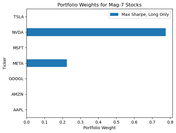
What if we want the actual, positive Sharpe ratio? We can use the Sharpe() function. If we want to update the results in res_1, we could write another helper function. However, I generally give in and learn to live with the output of commonly used functions.
res_1 message: Optimization terminated successfully
success: True
status: 0
fun: -1.4135274708532686
x: [ 0.000e+00 0.000e+00 7.275e-17 2.248e-01 4.052e-17
7.752e-01 4.228e-17]
nit: 6
jac: [ 1.533e-01 3.427e-01 2.659e-01 -4.758e-05 2.516e-01
1.378e-05 3.652e-01]
nfev: 48
njev: 6Sharpe(w=res_1['x'], Sigma_excess=Sigma_excess, mu_excess=mu_excess)1.4135Find the maximum Sharpe Ratio portfolio of Mag 7 stocks over the last three years, but allow short weights up to 10% on each stock
We can short 6 of 7 stocks up to -0.1 for a total of -0.6. Therefore, the maximum possible long weight is 1.6, and bounds becomes:
bounds=[(-0.1, 1.6) for _ in range(7)],res_2 = sco.minimize(
fun=Sharpe_neg,
x0=equal_weights(Sigma_excess.shape[1]),
args=(Sigma_excess, mu_excess),
bounds=[(-0.1, 1.6) for _ in range(7)],
constraints=(
{'type': 'eq', 'fun': lambda x: x.sum() - 1}
)
)res_df['Max Sharpe, Short up to 10% Each'] = res_2['x']res_df.plot(kind='barh')
plt.title('Portfolio Weights for Mag-7 Stocks')
plt.xlabel('Portfolio Weight')
plt.show()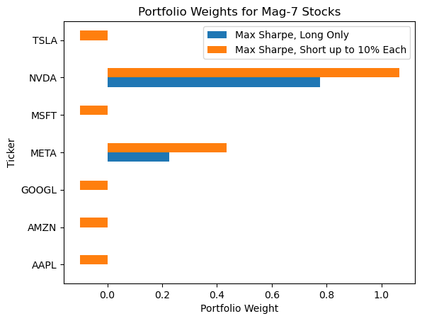
Find the maximum Sharpe Ratio portfolio of Mag 7 stocks over the last three years, but allow total short weights of up to 30%
We need to use an unequality constraints to make sure the sum of the negative portfolios weights is greater than -0.3. We express inequality constraints with functions with non-negative outputs, so we use \(\sum_i w_i[w_i < 0] + 0.3 \geq 0\).
We see that once we allow shorts greater than 30%, we spend almost all of this short budget on AMZN.
toy = np.arange(-2, 3)toy[toy < 0].sum()np.int64(-3)res_3 = sco.minimize(
fun=Sharpe_neg,
x0=equal_weights(Sigma_excess.shape[1]),
args=(Sigma_excess, mu_excess),
bounds=[(-0.3, 1.3) for _ in range(7)],
constraints=(
{'type': 'eq', 'fun': lambda x: x.sum() - 1},
{'type': 'ineq', 'fun': lambda x: x[x < 0].sum() + 0.3}
)
)res_df['Max Sharpe, Short up to 30% Total'] = res_3['x']res_df.plot(kind='barh')
plt.title('Portfolio Weights for Mag-7 Stocks')
plt.xlabel('Portfolio Weight')
plt.show()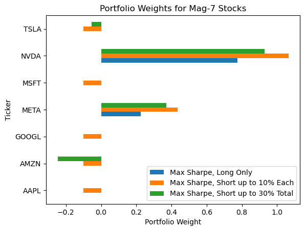
Find the maximum Sharpe Ratio portfolio of Mag 7 stocks over the last three years, but do not allow any weight to exceed 30% in magnitude
We can bound all portfolios weights on \([0, 0.3]\) with:
bounds=[(0, 0.3) for _ in range(7)]res_4 = sco.minimize(
fun=Sharpe_neg,
x0=equal_weights(Sigma_excess.shape[1]),
args=(Sigma_excess, mu_excess),
bounds=[(0, 0.3) for _ in range(7)],
constraints=(
{'type': 'eq', 'fun': lambda x: x.sum() - 1}
)
)res_df['Max Sharpe, Long Only up to 30% Each'] = res_4['x']res_df.plot(kind='barh')
plt.title('Portfolio Weights for Mag-7 Stocks')
plt.xlabel('Portfolio Weight')
plt.show()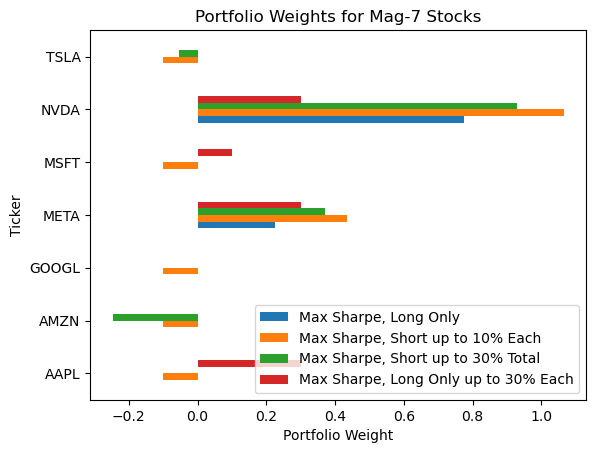
Find the minimum 95% Value at Risk (Var) portfolio of Mag 7 stocks over the last three years
More on VaR here.
def VaR(weights, returns, percent):
    return returns.dot(weights).quantile(1 - percent)
VaR(
weights=equal_weights(returns.shape[1]),
returns=returns,
percent=0.95
)-0.0338def VaR_neg(weights, returns, percent):
return -1 * VaR(weights=weights, returns=returns, percent=percent)res_var = sco.minimize(
fun=VaR_neg,
x0=equal_weights(returns.shape[1]), # np.ones(7) / 7
args=(returns, 0.95),
bounds=[(0, 1) for _ in range(returns.shape[1])],
constraints=(
{'type': 'eq', 'fun': lambda w: w.sum() - 1}
)
)res_df['Minimum 1-Day 95% VaR'] = res_var['x']res_df.plot(kind='barh')
plt.title('Portfolio Weights for Mag-7 Stocks')
plt.xlabel('Portfolio Weight')
plt.show()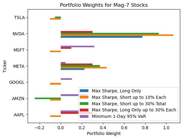
Find the minimum draw down portfolio of Mag 7 stocks over the last three years
def Max_Drawdown(w, returns):
    price = returns.dot(w).add(1).cumprod()
return (price / price.cummax() - 1).min()Max_Drawdown(equal_weights(7), returns)-0.3942The maximum drawdown is a negative number, but we want the smallest negative number, so we minimize negative one times the maximum drawdown.
def Max_Drawdown_neg(w, returns):
    return -1 * Max_Drawdown(w=w, returns=returns)
res_mdd = sco.minimize(
fun=Max_Drawdown_neg,
x0=equal_weights(returns.shape[1]), # np.ones(7) / 7
args=(returns,),
bounds=[(0, 1) for _ in range(returns.shape[1])],
constraints=(
{'type': 'eq', 'fun': lambda w: w.sum() - 1}
)
)res_df['Min Max Drawdown'] = res_mdd['x']res_df.plot(kind='barh')
plt.title('Portfolio Weights for Mag-7 Stocks')
plt.xlabel('Portfolio Weight')
plt.show()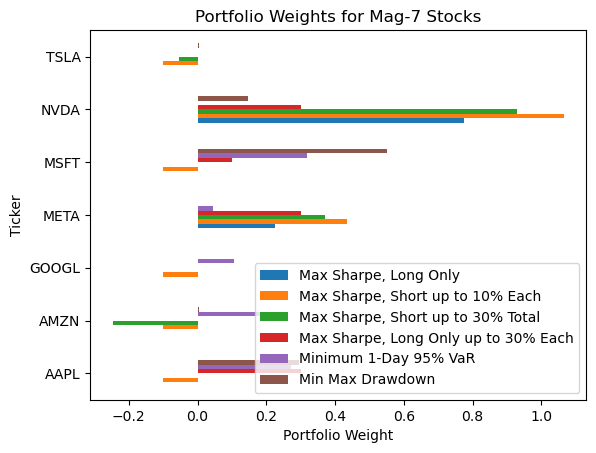
Find the minimum draw down portfolio for the sample with complete data for the current Dow-Jones Industrial Average (DJIA) stocks
You can find the DJIA tickers on Wikipedia.
tickers = (
    pd.read_html(io='https://en.wikipedia.org/wiki/Dow_Jones_Industrial_Average')
    [2]
    ['Symbol']
    .to_list()
)
djia = (
yf.download(
tickers=tickers,
auto_adjust=False,
progress=False
)
.iloc[:-1]
['Adj Close']
.pct_change()
.dropna()
)res_mdd = sco.minimize(
fun=Max_Drawdown_neg,
x0=equal_weights(djia.shape[1]),
args=(djia,),
bounds=[(0, 1) for _ in range(djia.shape[1])],
constraints=(
{'type': 'eq', 'fun': lambda w: w.sum() - 1}
)
)res_djia = pd.DataFrame(
data={'Min Max Drawdown': res_mdd['x']},
index=djia.columns
)res_djia.plot(kind='barh')
plt.title('Portfolio Weights for DJIA Stocks')
plt.xlabel('Portfolio Weight')
plt.show()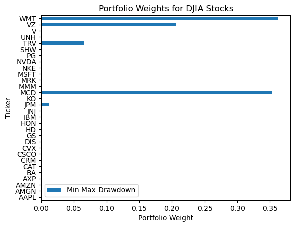
Plot the minimum-variance frontier for the sample with complete data for the current the DJIA stocks
See the lecture notebook for a similar exercise with the Mag-7 stocks.
def calc_sigmap(w, Sigma, ppy=252):
return np.sqrt(ppy * w.T @ Sigma @ w)def calc_mup(w, mu, ppy=252):
return ppy * w.T @ muSigma = djia.cov()mu = djia.mean()djia_target = 252 * np.linspace(
start=mu.min(),
stop=mu.max(),
num=50
)res_ef = []
for r in djia_target:
_ = sco.minimize(
fun=calc_sigmap,
x0=np.ones(Sigma.shape[1]) / Sigma.shape[1],
args=(Sigma, 252),
bounds=[(0, 1) for c in Sigma.index],
constraints=(
{'type': 'eq', 'fun': lambda x: x.sum() - 1},
{'type': 'eq', 'fun': lambda x: calc_mup(w=x, mu=mu, ppy=252) - r}
)
)
res_ef.append(_)for r in res_ef:
assert r['success'] mv_frontier = pd.DataFrame({
'returns_target': djia_target,
'volatility': np.array([r['fun'] if r['success'] else np.nan for r in res_ef])
})(
mv_frontier
.mul(100)
.plot(x='volatility', y='returns_target', legend=False)
)
plt.ylabel('Annualized Mean Return (%)')
plt.xlabel('Annualized Volatility (%)')
for t in Sigma.index:
x = 100 * np.sqrt(252 * Sigma.loc[t, t])
y = 100 * 252 * mu.loc[t]
plt.annotate(text=t, xy=(x, y))
plt.show()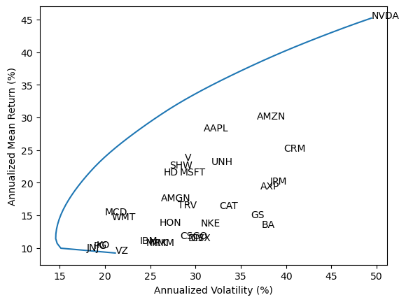
Find the maximum Sharpe Ratio portfolio for the sample with complete data for the current the DJIA stocks excluding the last three years, so we can compare to the 1/n portfolio to the maximum Sharpe ratio portfolio
This exercise is less dramatic withe NVDA this year. We will see three things:
- The maximum Sharpe ratio portfolio has a high Sharpe ratio in sample (or what we called
_beforein class) - But this same portfolio has a much lower Sharpe ratio out of sample (or what we called
_afterin class) - The 1/N or equal-weighted portfolio has about the same Sharpe ratio as the maximum Sharpe ratio portfolio out of sample
djia_excess = djia.sub(ff3['RF'], axis=0)
Sigma_excess_before = djia_excess.iloc[:-756].cov()
mu_excess_before = djia_excess.iloc[:-756].mean()Sigma_excess_after = djia_excess.iloc[-756:].cov()
mu_excess_after = djia_excess.iloc[-756:].mean()res_before = sco.minimize(
fun=Sharpe_neg,
x0=equal_weights(Sigma_excess_before.shape[1]),
args=(Sigma_excess_before, mu_excess_before),
bounds=[(0, 1) for _ in range(Sigma_excess_before.shape[1])],
constraints=(
{'type': 'eq', 'fun': lambda x: x.sum() - 1}
)
)The maximum Sharpe ratio portfolio has a high Sharpe ratio in sample!
Sharpe(
w=res_before['x'],
Sigma_excess=Sigma_excess_before,
mu_excess=mu_excess_before,
ppy=252
)1.2248res_djia[‘Max Sharpe Ratio 2008–2022’] = res_before[‘x’]
res_djia.plot(kind='barh')
plt.title('Portfolio Weights for DJIA Stocks')
plt.xlabel('Portfolio Weight')
plt.show()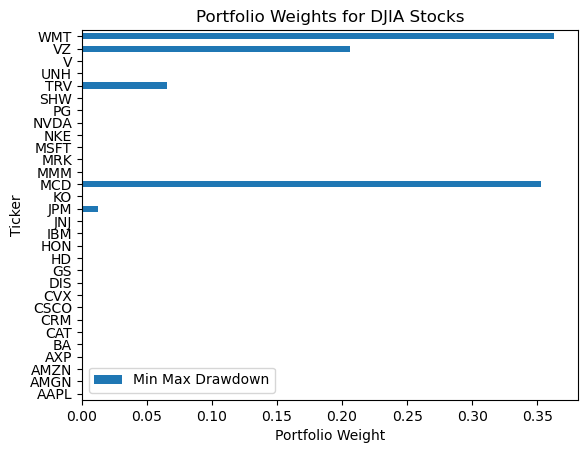
The maximum Sharpe ratio portfolio has a much lower Sharpe ratio out of sample!
Sharpe(
    w=res_before['x'],
    Sigma_excess=Sigma_excess_after,
    mu_excess=mu_excess_after,
    ppy=252
)0.7713Furthermore, the 1/N or equal-weighted portfolio does about as well out of sample!
Sharpe(
    w=equal_weights(Sigma_excess_after.shape[1]),
    Sigma_excess=Sigma_excess_after,
    mu_excess=mu_excess_after,
    ppy=252
)
0.6718