import matplotlib.pyplot as plt
import numpy as np
import pandas as pd
import pandas_datareader as pdr
import yfinance as yfMcKinney Chapter 10 - Practice - Sec 04
FINA 6333 for Spring 2025
%precision 4
pd.options.display.float_format = '{:.4f}'.format
# %config InlineBackend.figure_format = 'retina'
Announcements
- Please join your project group today. Otherwise, I will randomly assign you to a group tonight.
- Please vote for students’ choice topics.
- Please complete a week-5 survey; see the announcement on Canvas.
Five-Minute Review
We will focus on 3 topics from chapter 10 of McKinney:
- GroupBy Mechanics: We will use the
.groupby()method to perform “split-apply-combine” calculations in pandas, which let us aggregate data by one of more columns or indexes. - Data Aggregation: We will combine optimized methods, like
.count(),.sum(),.mean(), etc., with.groupby()to quickly aggregate data. We will combine the.agg()or.aggregate()method with.groupby()when we want to apply more than one aggregation function. - Pivot Tables: We can use the
.pivot_table()method to aggregate data with a syntax similar to Excel’s pivot tables. We can almost always get the same output with the.groupby(),.agg(), and.unstack()methods.
Practice
Replicate the following .pivot_table() output with .groupby()
ind = (
    yf.download(
        tickers='^GSPC ^DJI ^IXIC ^FTSE ^N225 ^HSI',
        auto_adjust=False,
        progress=False
    )
    .iloc[:-1]
    .stack(future_stack=True)
)
Tip
I learned after class that pd.Grouper() now has a level argument, too! We do not have to reset a data frame index just to use pd.Grouper()!
# Filter rows from 2015 onward
# Then pivot the 'ind' DataFrame so that:
#   - 'Close' values are aggregated
#   - Rows (index) are grouped yearly by 'Date' via pd.Grouper(...)
#   - Columns are broken out by 'Ticker'
#   - Both the 'min' and 'max' of 'Close' are calculated for each Ticker-year
# NOTE: pd.Grouper(level='Date', freq='YE') groups rows by the 'Date' index,
#       rolling them up to the 'Year-End' frequency.
a = (
    ind
    .loc['2015':]
    .pivot_table(
        values='Close',
        index=pd.Grouper(level='Date', freq='YE'),
        columns='Ticker',
        aggfunc=['min', 'max']
    )
)a.head()| min | max | |||||||||||
|---|---|---|---|---|---|---|---|---|---|---|---|---|
| Ticker | ^DJI | ^FTSE | ^GSPC | ^HSI | ^IXIC | ^N225 | ^DJI | ^FTSE | ^GSPC | ^HSI | ^IXIC | ^N225 |
| Date | ||||||||||||
| 2015-12-31 | 15666.4404 | 5874.1001 | 1867.6100 | 20556.5996 | 4506.4902 | 16795.9609 | 18312.3906 | 7104.0000 | 2130.8201 | 28442.7500 | 5218.8599 | 20868.0293 |
| 2016-12-31 | 15660.1797 | 5537.0000 | 1829.0800 | 18319.5801 | 4266.8398 | 14952.0195 | 19974.6191 | 7142.7998 | 2271.7200 | 24099.6992 | 5487.4399 | 19494.5293 |
| 2017-12-31 | 19732.4004 | 7099.2002 | 2257.8301 | 22134.4707 | 5429.0801 | 18335.6309 | 24837.5098 | 7687.7998 | 2690.1599 | 30003.4902 | 6994.7598 | 22939.1797 |
| 2018-12-31 | 21792.1992 | 6584.7002 | 2351.1001 | 24585.5293 | 6192.9199 | 19155.7402 | 26828.3906 | 7877.5000 | 2930.7500 | 33154.1211 | 8109.6899 | 24270.6191 |
| 2019-12-31 | 22686.2207 | 6692.7002 | 2447.8899 | 25064.3594 | 6463.5000 | 19561.9609 | 28645.2598 | 7686.6001 | 3240.0200 | 30157.4902 | 9022.3896 | 24066.1191 |
# Filter rows from 2015 onward.
# Group by both:
#    1) Year-end frequency of the 'Date' index (pd.Grouper(level='Date', freq='YE')), and
#    2) 'Ticker'.
# Then select the 'Close' column from each group and aggregate by taking
# the 'min' and 'max'. Finally, use .unstack() to move 'Ticker' back to columns.
b = (
    ind
    .loc['2015':]
    .groupby([pd.Grouper(level='Date', freq='YE'), 'Ticker'])
    ['Close']
    .agg(['min', 'max'])
    .unstack()
)a.equals(b)Truenp.allclose(a, b)True(a == b).all().all()np.True_Calulate the mean and standard deviation of returns by ticker for the MATANA (MSFT, AAPL, TSLA, AMZN, NVDA, and GOOG) stocks
Consider only dates with complete returns data. Try this calculation with wide and long data frames, and confirm your results are the same.
matana = (
    yf.download(
        tickers='MSFT AAPL TSLA AMZN NVDA GOOG',
        auto_adjust=False,
        progress=False
    )
    .iloc[:-1]
)
columns = pd.MultiIndex.from_product([['Return'], matana['Adj Close'].columns])
matana[columns] = matana['Adj Close'].pct_change()matana['Return'].dropna().agg(['mean', 'std'])| Ticker | AAPL | AMZN | GOOG | MSFT | NVDA | TSLA |
|---|---|---|---|---|---|---|
| mean | 0.0011 | 0.0012 | 0.0009 | 0.0010 | 0.0021 | 0.0021 |
| std | 0.0175 | 0.0205 | 0.0173 | 0.0161 | 0.0288 | 0.0362 |
Homework! Re-do this aggregation with annualized* means and volatilities!*
We have (at least) two options here.
- Write functions that calculate annualized means and volatilities, say
ann_mean()andann_std() - Use lambda (anonymous functions), then rename the rows
First, here is the “write functions” solution. We do not need to provide userr-written function names in quotes.
def ann_mean(x, ann_fac=252):
    return ann_fac * x.mean()
def ann_std(x, ann_fac=np.sqrt(252)):
return ann_fac * x.std()a = matana['Return'].agg([ann_mean, ann_std])
a| Ticker | AAPL | AMZN | GOOG | MSFT | NVDA | TSLA |
|---|---|---|---|---|---|---|
| ann_mean | 0.2748 | 0.4294 | 0.2528 | 0.2816 | 0.4888 | 0.5175 |
| ann_std | 0.4406 | 0.5583 | 0.3061 | 0.3336 | 0.6004 | 0.5740 |
Second, here is the “lambda functions” solution.
b = matana['Return'].agg([lambda x: 252*x.mean(), lambda x: np.sqrt(252)*x.std()])
b.index = ['Mean', 'Volatility']
b| Ticker | AAPL | AMZN | GOOG | MSFT | NVDA | TSLA |
|---|---|---|---|---|---|---|
| Mean | 0.2748 | 0.4294 | 0.2528 | 0.2816 | 0.4888 | 0.5175 |
| Volatility | 0.4406 | 0.5583 | 0.3061 | 0.3336 | 0.6004 | 0.5740 |
np.allclose(a=a, b=b)True(These values differ just enough that we have to complete the fuzzy equality of np.allclose() instead of the exact equality of .equals().)
Calculate the mean and standard deviation of returns and the maximum of closing prices by ticker for the MATANA stocks
We have to reshape our data first, because the .agg() method does not work well with column multi-indexes. The .rename_axis() method is optional, but I prefer to name my axes to simplify later stacking and unstacking.
a = (
    matana
    .stack(future_stack=True)
    .groupby(level='Ticker')
    .agg({
        'Return': ['mean', 'std'],
        'Close': 'max'
    })
    .rename_axis(columns=['Variable', 'Statistic'])
)
a| Variable | Return | Close | |
|---|---|---|---|
| Statistic | mean | std | max |
| Ticker | |||
| AAPL | 0.0011 | 0.0278 | 259.0200 |
| AMZN | 0.0017 | 0.0352 | 242.0600 |
| GOOG | 0.0010 | 0.0193 | 207.7100 |
| MSFT | 0.0011 | 0.0210 | 467.5600 |
| NVDA | 0.0019 | 0.0378 | 149.4300 |
| TSLA | 0.0021 | 0.0362 | 479.8600 |
We can do the same operation with .pivot_table().
b = (
    matana
    .stack(future_stack=True)
    .pivot_table(
        index='Ticker',
        aggfunc={
        'Return': ['mean', 'std'],
        'Close': 'max'
    }
))
b| Price | Close | Return | |
|---|---|---|---|
| max | mean | std | |
| Ticker | |||
| AAPL | 259.0200 | 0.0011 | 0.0278 |
| AMZN | 242.0600 | 0.0017 | 0.0352 |
| GOOG | 207.7100 | 0.0010 | 0.0193 |
| MSFT | 467.5600 | 0.0011 | 0.0210 |
| NVDA | 149.4300 | 0.0019 | 0.0378 |
| TSLA | 479.8600 | 0.0021 | 0.0362 |
The column orders differ between .agg() and .pivot_table() solutions, but the values are the same.
a[['Close', 'Return']].equals(b[['Close', 'Return']])TrueCalculate monthly means and volatilities for SPY and GOOG returns
spy_goog = (
    yf.download(
        tickers='SPY GOOG',
        auto_adjust=False,
        progress=False
    )
    .iloc[:-1]
)

spy_goog| Price | Adj Close | Close | High | Low | Open | Volume | ||||||
|---|---|---|---|---|---|---|---|---|---|---|---|---|
| Ticker | GOOG | SPY | GOOG | SPY | GOOG | SPY | GOOG | SPY | GOOG | SPY | GOOG | SPY |
| Date | ||||||||||||
| 1993-01-29 | NaN | 24.5261 | NaN | 43.9375 | NaN | 43.9688 | NaN | 43.7500 | NaN | 43.9688 | NaN | 1003200 |
| 1993-02-01 | NaN | 24.7005 | NaN | 44.2500 | NaN | 44.2500 | NaN | 43.9688 | NaN | 43.9688 | NaN | 480500 |
| 1993-02-02 | NaN | 24.7528 | NaN | 44.3438 | NaN | 44.3750 | NaN | 44.1250 | NaN | 44.2188 | NaN | 201300 |
| 1993-02-03 | NaN | 25.0145 | NaN | 44.8125 | NaN | 44.8438 | NaN | 44.3750 | NaN | 44.4062 | NaN | 529400 |
| 1993-02-04 | NaN | 25.1192 | NaN | 45.0000 | NaN | 45.0938 | NaN | 44.4688 | NaN | 44.9688 | NaN | 531500 |
| ... | ... | ... | ... | ... | ... | ... | ... | ... | ... | ... | ... | ... |
| 2025-02-21 | 181.5800 | 599.9400 | 181.5800 | 599.9400 | 187.4700 | 610.3000 | 181.1300 | 599.4700 | 187.2900 | 610.1600 | 19520800.0000 | 76519800 |
| 2025-02-24 | 181.1900 | 597.2100 | 181.1900 | 597.2100 | 185.0900 | 603.0300 | 180.8800 | 596.4900 | 183.8000 | 602.0200 | 18734000.0000 | 50737200 |
| 2025-02-25 | 177.3700 | 594.2400 | 177.3700 | 594.2400 | 180.7600 | 597.8900 | 176.7700 | 589.5600 | 180.1550 | 597.1500 | 20832500.0000 | 58266500 |
| 2025-02-26 | 174.7000 | 594.5400 | 174.7000 | 594.5400 | 178.0800 | 599.5800 | 173.5900 | 591.8600 | 176.9450 | 595.9300 | 23637200.0000 | 43321600 |
| 2025-02-27 | 170.2100 | 585.0500 | 170.2100 | 585.0500 | 176.5900 | 598.0200 | 169.7520 | 584.6500 | 175.9400 | 596.8500 | 25930500.0000 | 74196700 |
8076 rows × 12 columns
spy_goog_m = (
    spy_goog
    ['Adj Close']
    .pct_change()
    .groupby(pd.Grouper(level='Date', freq='ME'))
    .agg(['mean', 'std'])
    .dropna(how='all')
    .rename_axis(columns=['Ticker', 'Statistic'])
)

spy_goog_m| Ticker | GOOG | SPY | ||
|---|---|---|---|---|
| Statistic | mean | std | mean | std |
| Date | ||||
| 1993-02-28 | NaN | NaN | 0.0006 | 0.0080 |
| 1993-03-31 | NaN | NaN | 0.0010 | 0.0071 |
| 1993-04-30 | NaN | NaN | -0.0012 | 0.0074 |
| 1993-05-31 | NaN | NaN | 0.0014 | 0.0071 |
| 1993-06-30 | NaN | NaN | 0.0002 | 0.0060 |
| ... | ... | ... | ... | ... |
| 2024-10-31 | 0.0015 | 0.0126 | -0.0004 | 0.0070 |
| 2024-11-30 | -0.0005 | 0.0191 | 0.0029 | 0.0075 |
| 2024-12-31 | 0.0056 | 0.0223 | -0.0011 | 0.0090 |
| 2025-01-31 | 0.0040 | 0.0167 | 0.0014 | 0.0088 |
| 2025-02-28 | -0.0102 | 0.0207 | -0.0015 | 0.0075 |
385 rows × 4 columns
Plot the monthly means and volatilities from the previous exercise
Let us try .plot() first!
spy_goog_m.plot()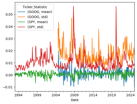
This plot is not very useful because:
- Mean and volatility are on the same y axis
- The legend title and labels are cluttered
Let use try the subplots=True argument to .plot().
spy_goog_m.plot(subplots=True)array([<Axes: xlabel='Date'>, <Axes: xlabel='Date'>,
<Axes: xlabel='Date'>, <Axes: xlabel='Date'>], dtype=object)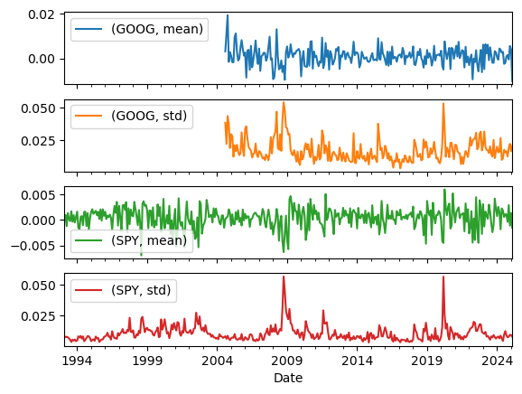
This plot is slightly better, but once I need a more complex plot with different statistics and different individuals, I switch to seaborn. seaborn is a plotting package built on top of matplotlib and does an excellent job with different statistics and different individuals. The following example uses sns.replot() to plot these four series. seaborn works best with all y values in one column, which we might call and really long data frame, and columns instead of indexes. Please see my comments on the code below.
import seaborn as sns(
# Start with the 'spy_goog_m' DataFrame that contains monthly volatility and returns for SPY and GOOG
spy_goog_m
# Stack the DataFrame once; by default stack will pivot the inner column index into the row index
.stack(future_stack=True)
# Stack a second time to fully pivot all remaining columns into the index
.stack(future_stack=True)
# Convert the stacked Series into a DataFrame and name the single value column as 'Value'
.to_frame('Value')
# Reset the multi-level index so that 'Date', 'Ticker', and 'Statistic' become columns
.reset_index()
# Use .pipe() to pass the resulting DataFrame directly into sns.relplot with the following arguments
.pipe(
sns.relplot,
x='Date', # The x-axis will be the 'Date' column
y='Value', # The y-axis will be the 'Value' column (volatility or returns)
hue='Ticker', # Different lines/colors for each ticker (SPY vs GOOG)
col='Statistic', # Create separate plots (facets) for each statistic (volatility or returns)
kind='line', # Plot a line chart
facet_kws={'sharey': False} # Allow each facet to have its own y-scale instead of sharing a single scale
)
)
plt.suptitle('Monthly Mean and Volatility of Daily Returns', y=1.02)
plt.show()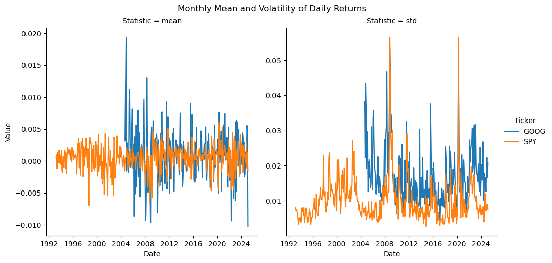
Assign the Dow Jones stocks to five portfolios based on the preceding month’s volatility
This example may make more sense after we cover chapter 11 on time-series tools. I recently added “preceding” to this example to prevent any look-ahead bias, but it makes this example more challenging.
First, we download DJIA data from Yahoo! Finance using the current DJIA tickers from Wikipedia.
wiki = pd.read_html('https://en.wikipedia.org/wiki/Dow_Jones_Industrial_Average')djia = (
yf.download(
tickers=wiki[2]['Symbol'].to_list(),
auto_adjust=False,
progress=False
)
.iloc[:-1]
)Next, we will calculate daily returns for djia. We have to use our pd.MultiIndex.from_product() trick to create a multi-index for the columns.
Tip
pd.MultiIndex.from_product() takes a list of iterables (e.g., lists or arrays) and creates all possible combinations of their elements. This combination is called a Cartesian product. Each unique combination becomes a distinct entry in the resulting multi index.
columns = pd.MultiIndex.from_product([['Return'], djia['Adj Close'].columns])
djia[columns] = djia['Adj Close'].pct_change()
Next, we calculate monthly volatility of daily returns, then assign stocks to portfolios based on these volatilities. We will keep these portfolio assignment separate from djia, for now. We use the .apply() method with axis=1 to apply pd.qcut to every row/month in without writing a for loop. We can also pass q=5 and labels=False after we give the pd.qcut function name. Here is a simple pd.qcut() example.
np.arange(10)array([0, 1, 2, 3, 4, 5, 6, 7, 8, 9])pd.qcut(
x=np.arange(10),
q=5,
labels=False
)array([0, 0, 1, 1, 2, 2, 3, 3, 4, 4])djia_portfolios = (
djia
['Return'] # Start with 'Return' data
.dropna() # Drop rows with missing values
.groupby(pd.Grouper(level='Date', freq='ME')) # Group by month-end
.std() # Compute std dev within each group
.apply(pd.qcut, q=5, labels=False, axis=1) # Bin into 5 quantiles
)
columns = pd.MultiIndex.from_product([['Portfolio'], djia['Return'].columns])
djia_portfolios.columns = columns
djia_portfolios.head()| Portfolio | |||||||||||||||||||||
|---|---|---|---|---|---|---|---|---|---|---|---|---|---|---|---|---|---|---|---|---|---|
| Ticker | AAPL | AMGN | AMZN | AXP | BA | CAT | CRM | CSCO | CVX | DIS | ... | MSFT | NKE | NVDA | PG | SHW | TRV | UNH | V | VZ | WMT |
| Date | |||||||||||||||||||||
| 2008-03-31 | 3 | 1 | 3 | 4 | 2 | 0 | 3 | 3 | 0 | 1 | ... | 2 | 4 | 3 | 0 | 2 | 1 | 2 | 4 | 2 | 2 |
| 2008-04-30 | 3 | 1 | 4 | 3 | 2 | 3 | 4 | 2 | 0 | 1 | ... | 3 | 1 | 4 | 0 | 2 | 2 | 4 | 3 | 1 | 0 |
| 2008-05-31 | 3 | 1 | 4 | 4 | 2 | 0 | 4 | 3 | 1 | 2 | ... | 2 | 2 | 4 | 0 | 3 | 2 | 3 | 4 | 2 | 1 |
| 2008-06-30 | 3 | 0 | 4 | 4 | 3 | 0 | 4 | 1 | 1 | 1 | ... | 2 | 4 | 3 | 0 | 2 | 2 | 2 | 3 | 2 | 1 |
| 2008-07-31 | 2 | 3 | 4 | 4 | 2 | 2 | 2 | 1 | 1 | 1 | ... | 2 | 1 | 4 | 0 | 4 | 3 | 3 | 4 | 0 | 1 |
5 rows × 30 columns
Combining the returns and portfolios is the trickiest step because we want to prevent a look-ahead bias. For example, we do not know that AAPL is in portfolio 3 until March 2008 ends. Therefore, AAPL cannot be in portfolio 3 until April 2008!
djia_w_portfolios = djia.join(djia_portfolios.shift(periods=1, freq='D'))
djia_w_portfolios['Portfolio'] = djia_w_portfolios['Portfolio'].ffill()
Plot the time-series volatilities of these five portfolios
(
    djia_w_portfolios                  # start data frame with portfolio assignments
    .stack(future_stack=True)          # Reshape columns into rows
    .dropna()                          # Remove rows with missing values
    .groupby([pd.Grouper(level='Date', freq='ME'), 'Portfolio'])  # Group by month-end & portfolio
    ['Return']                         # Operate on 'Return'
    .std()                             # Calculate std dev for each group
    .to_frame('Volatility')            # Convert to DataFrame named 'Volatility'
    .reset_index()                     # Make grouped cols into normal columns to fix portfolio colums
    .assign(Portfolio=lambda x: x['Portfolio'].astype(int) + 1)  # Convert portfolio to int & increment
    .set_index(['Date', 'Portfolio'])  # Use 'Date' & 'Portfolio' as new index
    .unstack()['Volatility']           # Reshape wide, focusing on 'Volatility'
    .plot()                            # Generate the plot
)

plt.title('Volatility of Equal-Weighted Portfolios\n Portfolios Formed on Previous Month\'s Volatility')
plt.ylabel('Monthly Volatility of Daily Portfolio Returns')
plt.show()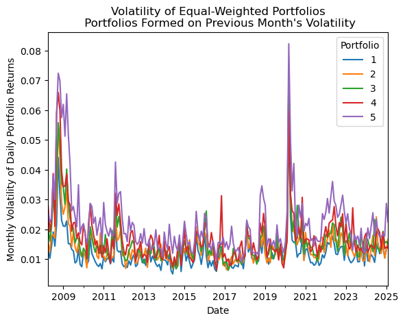
Calculate the mean monthly correlation between the Dow Jones stocks
We will keep any day with at least 20 stocks. 20 is an arbitrary threshold but provides a 40+ year sample. The thresh=20 argument to the .dropna() method drops any row with fewer than 20 non-missing values.
djia['Return'].dropna(thresh=20).count(axis=1)Date
1981-09-23 20
1981-09-24 20
1981-09-25 20
1981-09-28 20
1981-09-29 20
..
2025-02-21 30
2025-02-24 30
2025-02-25 30
2025-02-26 30
2025-02-27 30
Length: 10947, dtype: int64Then we can use the axis=1 argument to the .dropna() to drop any stocks without data.
djia['Return'].dropna(thresh=20).dropna(axis=1).count()Ticker
AAPL 10947
AXP 10947
BA 10947
CAT 10947
CVX 10947
DIS 10947
HD 10947
HON 10947
IBM 10947
JNJ 10947
JPM 10947
KO 10947
MCD 10947
MMM 10947
MRK 10947
NKE 10947
PG 10947
SHW 10947
TRV 10947
WMT 10947
dtype: int64Next, we calculate the pairwise correlations between every stock every month.
(
    djia['Return']
    .dropna(thresh=20)
    .dropna(axis=1)
    .groupby(pd.Grouper(level='Date', freq='ME'))
    .corr()
)| Ticker | AAPL | AXP | BA | CAT | CVX | DIS | HD | HON | IBM | JNJ | JPM | KO | MCD | MMM | MRK | NKE | PG | SHW | TRV | WMT | |
|---|---|---|---|---|---|---|---|---|---|---|---|---|---|---|---|---|---|---|---|---|---|
| Date | Ticker | ||||||||||||||||||||
| 1981-09-30 | AAPL | 1.0000 | 0.6520 | 0.4549 | 0.5633 | 0.2316 | 0.8654 | NaN | 0.2991 | 0.1691 | -0.0721 | -0.0441 | 0.8272 | 0.3542 | 0.5247 | 0.6755 | 0.8195 | 0.7045 | 0.7338 | 0.6740 | 0.8170 |
| AXP | 0.6520 | 1.0000 | 0.8350 | 0.7389 | 0.4941 | 0.6656 | NaN | 0.7529 | 0.4243 | 0.6275 | -0.5158 | 0.8953 | 0.8155 | 0.6453 | 0.8543 | 0.2044 | 0.9348 | 0.8512 | 0.0686 | 0.5737 | |
| BA | 0.4549 | 0.8350 | 1.0000 | 0.5696 | 0.8357 | 0.6053 | NaN | 0.9685 | 0.7334 | 0.7441 | -0.5713 | 0.6188 | 0.9314 | 0.4350 | 0.9594 | 0.0042 | 0.7765 | 0.8539 | 0.0741 | 0.1810 | |
| CAT | 0.5633 | 0.7389 | 0.5696 | 1.0000 | 0.0854 | 0.2721 | NaN | 0.6128 | 0.6238 | 0.1520 | -0.5054 | 0.8419 | 0.3352 | 0.0391 | 0.5817 | 0.4289 | 0.5807 | 0.8575 | -0.1149 | 0.4428 | |
| CVX | 0.2316 | 0.4941 | 0.8357 | 0.0854 | 1.0000 | 0.5229 | NaN | 0.7683 | 0.5997 | 0.7313 | -0.5092 | 0.1714 | 0.8648 | 0.3567 | 0.8018 | -0.2339 | 0.4587 | 0.5080 | 0.1337 | -0.1611 | |
| ... | ... | ... | ... | ... | ... | ... | ... | ... | ... | ... | ... | ... | ... | ... | ... | ... | ... | ... | ... | ... | ... |
| 2025-02-28 | NKE | 0.3162 | 0.0004 | 0.0482 | 0.0244 | 0.2118 | 0.1206 | 0.1274 | 0.6006 | 0.3535 | 0.2012 | -0.2302 | -0.0567 | 0.0871 | 0.1481 | 0.1327 | 1.0000 | 0.1820 | -0.0391 | 0.1860 | 0.0821 |
| PG | -0.1369 | -0.3545 | 0.0515 | -0.2272 | -0.1965 | -0.2196 | 0.0334 | 0.2961 | 0.0140 | 0.4862 | -0.0485 | 0.4350 | 0.1009 | -0.2339 | 0.3593 | 0.1820 | 1.0000 | 0.1759 | 0.4297 | 0.1360 | |
| SHW | -0.0145 | 0.4445 | -0.0237 | 0.4848 | -0.1259 | 0.0197 | 0.7095 | 0.0105 | -0.0923 | 0.1010 | 0.1241 | 0.0544 | -0.0392 | 0.3584 | -0.1950 | -0.0391 | 0.1759 | 1.0000 | 0.2488 | 0.4282 | |
| TRV | 0.0950 | 0.0765 | 0.4173 | 0.2083 | 0.0119 | 0.2739 | 0.2077 | 0.0778 | -0.1450 | 0.4844 | 0.0087 | -0.0008 | 0.1697 | 0.4362 | 0.3460 | 0.1860 | 0.4297 | 0.2488 | 1.0000 | 0.2788 | |
| WMT | 0.0765 | 0.2785 | 0.5015 | 0.2344 | -0.0594 | -0.0354 | 0.4986 | 0.0966 | -0.0319 | 0.0655 | 0.4388 | 0.1360 | 0.2373 | 0.3700 | -0.3174 | 0.0821 | 0.1360 | 0.4282 | 0.2788 | 1.0000 |
10440 rows × 20 columns
The hard part is to drop the duplicate and self correlations. The ssimplest solution is to .stack() this data frame, then only keep observations where the first tickers is alphabetically before the second ticker.
# Calculate correlations for each month-end, then reshape into a long format
djia_correlations = (
    djia['Return']                               # Start with daily returns
    .dropna(thresh=20)                           # Keep rows with at least 20 non-NA tickers
    .dropna(axis=1)                              # Drop any tickers that still have missing values
    .groupby(pd.Grouper(level='Date', freq='ME'))  # Group by end of each month
    .corr()                                      # Calculate correlation matrix for each month
    .stack()                                     # Convert from wide to long format
    .to_frame('Correlation')                     # Name the single column 'Correlation'
)

# Rename index levels for clarity
djia_correlations.index.names = ['Date', 'Ticker1', 'Ticker2']

# Compute mean monthly correlation, excluding the first/last partial months
mean_monthly_corr = (
    djia_correlations
    .iloc[1:-1]                 # Drop the first and last rows (partial months)
    .query('Ticker1 < Ticker2') # Keep only the upper triangle pairs
    .groupby('Date')            # Group by month
    .mean()                     # Average correlation across all ticker pairs
)

# Plot the mean correlation across time
mean_monthly_corr.plot(legend=False)
plt.ylabel('Mean Monthly Correlation of Daily Returns')
plt.title('Correlation of Dow-Jones Industrial Average Stocks\n(Current constituents, at least 20 stocks per month)')
plt.show()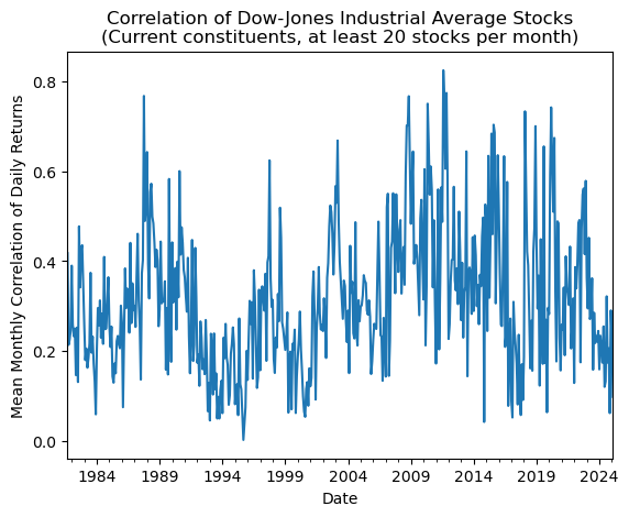
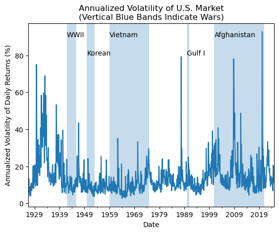
Is market volatility higher during wars?
Here is some guidance:
- Download the daily factor data from Ken French’s website
- Calculate daily market returns by summing the market risk premium and risk-free rates (
Mkt-RFandRF, respectively) - Calculate the volatility (standard deviation) of daily returns every month by combining
pd.Grouper()and.groupby()) - Multiply by \(\sqrt{252}\) to annualize these volatilities of daily returns
- Plot these annualized volatilities
Is market volatility higher during wars? Consider the following dates:
- WWII: December 1941 to September 1945
- Korean War: 1950 to 1953
- Viet Nam War: 1959 to 1975
- Gulf War: 1990 to 1991
- War in Afghanistan: 2001 to 2021
pdr.famafrench.get_available_datasets()[:5]['F-F_Research_Data_Factors',
'F-F_Research_Data_Factors_weekly',
'F-F_Research_Data_Factors_daily',
'F-F_Research_Data_5_Factors_2x3',
'F-F_Research_Data_5_Factors_2x3_daily']ff = pdr.DataReader(
name='F-F_Research_Data_Factors_daily',
data_source='famafrench',
start='1900'
)C:\Users\r.herron\AppData\Local\Temp\ipykernel_13148\875599436.py:1: FutureWarning: The argument 'date_parser' is deprecated and will be removed in a future version. Please use 'date_format' instead, or read your data in as 'object' dtype and then call 'to_datetime'.
ff = pdr.DataReader(# Calculate and plot the annualized daily volatility of the U.S. market
(
ff[0]
.assign(Mkt=lambda df: df['Mkt-RF'] + df['RF']) # Create 'Mkt' by adding market excess return + risk-free rate
['Mkt'] # Select only the 'Mkt' column
.groupby(pd.Grouper(freq='ME')) # Group by month-end
.std() # Compute standard deviation within each month
.mul(np.sqrt(252)) # Convert to annualized volatility (approx 252 trading days/yr)
.plot() # Plot the resulting monthly series
)
# Add vertical spans (blue bands) for U.S. wars, with annotation labels
plt.axvspan('1941-12', '1945-09', alpha=0.25)
plt.annotate('WWII', ('1941-12', 90))
plt.axvspan('1950', '1953', alpha=0.25)
plt.annotate('Korean', ('1950', 80))
plt.axvspan('1959', '1975', alpha=0.25)
plt.annotate('Vietnam', ('1959', 90))
plt.axvspan('1990', '1991', alpha=0.25)
plt.annotate('Gulf I', ('1990', 80))
plt.axvspan('2001', '2021', alpha=0.25)
plt.annotate('Afghanistan', ('2001', 90))
# Customize labels and title
plt.ylabel('Annualized Volatility of Daily Returns (%)')
plt.title('Annualized Volatility of U.S. Market\n(Vertical Blue Bands Indicate Wars)')
plt.show()