import matplotlib.pyplot as plt
import numpy as np
import pandas as pd
import pandas_datareader as pdr
import statsmodels.api as sm
import yfinance as yfHerron Topic 3 - Quantitative Value Investing
FINA 6333 for Spring 2025
%precision 4
pd.options.display.float_format = '{:.4f}'.format
# %config InlineBackend.figure_format = 'retina'
Introduction
This notebook adapts the portfolio formation approach from Fama and French (1993), who show that firms with high book-to-market equity ratios (value stocks) tend to outperform those with low ratios (growth stocks), forming the basis of the value factor in their three-factor model. This notebook relies on two large data files. You can find these files in our shared OneDrive folder or our Notebook and Syllabus folder on Canvas. These two files are:
- Firm-level market data (e.g., stock prices and share counts) from the Center for Research in Security Prices (CRSP) in
crsp.csv - Firm-level fundamentals (i.e., financial statement information) from Compustat in
compustat.csv
This notebook walks you through the steps to test a quantitative value investing strategy based on the book-to-market equity ratio (B/M). I based this lecture notebook on Gray and Carlisle (2012, chap. 1 and 7), which presents much more on quantitative value investing.
Import the data from CRSP and Compustat
CRSP
The CRSP data provide the following variables:
PERMNOis the stock identifierdateis the last trading day of the monthSHRCDindicates share class, and we can ignore itPRCis the share price in dollars, and negative prices indicate the price is the midpoint of the bid-ask spread instead of a transactionSHROUTis the number of shares outstanding in thousands
Read the CRSP data into a data frame named crsp. Be sure to parse dates. The codea A, B, and C indicate missing values.
crsp = (
    pd.read_csv(
        filepath_or_buffer='crsp.csv',
        parse_dates=['date'],
        na_values=list('ABC')
    )
    .query('date >= 1965')
    .sort_values(by=['PERMNO', 'date'])
    .assign(
        ME=lambda x: x['PRC'].abs() * x['SHROUT'] / 1000,
        date=lambda x: x['date'] + pd.offsets.MonthEnd(0)
    )
)crsp.head()| PERMNO | date | SHRCD | PRC | RET | SHROUT | ME | |
|---|---|---|---|---|---|---|---|
| 0 | 10000 | 1986-01-31 | 10 | -4.3750 | NaN | 3680.0000 | 16.1000 |
| 1 | 10000 | 1986-02-28 | 10 | -3.2500 | -0.2571 | 3680.0000 | 11.9600 |
| 2 | 10000 | 1986-03-31 | 10 | -4.4375 | 0.3654 | 3680.0000 | 16.3300 |
| 3 | 10000 | 1986-04-30 | 10 | -4.0000 | -0.0986 | 3793.0000 | 15.1720 |
| 4 | 10000 | 1986-05-31 | 10 | -3.1094 | -0.2227 | 3793.0000 | 11.7939 |
Compustat
The Compustat data provide the following variables:
GVKEYis the S&P firm identifierLPERMNOis the link between CRSP and Compustatdatadateis the date of the filing, which is the last day of the fiscal yearfyearis the fiscal yearceqis the book value of equityibis income before extraordinary items- We can ignore the other variables that Wharton Research Data Services (WRDS) adds to this data set
Read the Compustat data into a data frame named compustat. Be sure to parse dates.
compustat = (
    pd.read_csv(
        filepath_or_buffer='compustat.csv',
        parse_dates=['datadate']
    )
    .query('datadate >= 1965')
    .sort_values(['LPERMNO', 'fyear', 'datadate'])
    .drop_duplicates(subset=['LPERMNO', 'fyear'], keep='last')
)compustat.head()| GVKEY | LPERMNO | datadate | fyear | indfmt | consol | popsrc | datafmt | curcd | ceq | ib | costat | |
|---|---|---|---|---|---|---|---|---|---|---|---|---|
| 165681 | 13007 | 10000 | 1986-10-31 | 1986.0000 | INDL | C | D | STD | USD | 0.4180 | -0.7300 | I |
| 165586 | 12994 | 10001 | 1986-06-30 | 1986.0000 | INDL | C | D | STD | USD | 5.4320 | 0.6690 | I |
| 165587 | 12994 | 10001 | 1987-06-30 | 1987.0000 | INDL | C | D | STD | USD | 5.3690 | 0.3120 | I |
| 165588 | 12994 | 10001 | 1988-06-30 | 1988.0000 | INDL | C | D | STD | USD | 5.5120 | 0.5420 | I |
| 165589 | 12994 | 10001 | 1989-06-30 | 1989.0000 | INDL | C | D | STD | USD | 6.3210 | 1.2080 | I |
Create interim data frames
To test the book/market investing strategy, we need to match the following data:
- Book value of equity for year \(t-1\)
- Market value of equity from December of year \(t-1\)
- Portfolios for year \(t\) based on book and market values of equity in year \(t-1\)
- Returns from July of year \(t\) through June of year \(t+1\)
We will form portfolios once a year because the book value of equity updates once a year. Fama and French (1993) wait until June of year \(t\) to form portfolios, ensuring financial data from year \(t-1\) is public, then track returns from July in year \(t\) through June in year \(t+1\). The simplest and clearest way to match these data is to create one data frame for each of these three data sets.
Market value of equity from December of year \(t-1\)
Then create a new data frame mve that contains the latest market value of equity as of December.
mve = (
    crsp
    .query('ME > 0')
    .groupby(['PERMNO', pd.Grouper(key='date', freq='YE-DEC')])
    [['ME']]
    .last()
)crsp.query('PERMNO == 10001').head(12)| PERMNO | date | SHRCD | PRC | RET | SHROUT | ME | |
|---|---|---|---|---|---|---|---|
| 18 | 10001 | 1986-01-31 | 11 | -6.1250 | NaN | 985.0000 | 6.0331 |
| 19 | 10001 | 1986-02-28 | 11 | -6.2500 | 0.0204 | 985.0000 | 6.1562 |
| 20 | 10001 | 1986-03-31 | 11 | -6.3125 | 0.0252 | 985.0000 | 6.2178 |
| 21 | 10001 | 1986-04-30 | 11 | -6.3750 | 0.0099 | 985.0000 | 6.2794 |
| 22 | 10001 | 1986-05-31 | 11 | -6.3125 | -0.0098 | 985.0000 | 6.2178 |
| 23 | 10001 | 1986-06-30 | 11 | -6.1250 | -0.0131 | 985.0000 | 6.0331 |
| 24 | 10001 | 1986-07-31 | 11 | -6.0625 | -0.0102 | 985.0000 | 5.9716 |
| 25 | 10001 | 1986-08-31 | 11 | -6.5000 | 0.0722 | 985.0000 | 6.4025 |
| 26 | 10001 | 1986-09-30 | 11 | 6.3750 | -0.0031 | 991.0000 | 6.3176 |
| 27 | 10001 | 1986-10-31 | 11 | 6.6250 | 0.0392 | 991.0000 | 6.5654 |
| 28 | 10001 | 1986-11-30 | 11 | 7.0000 | 0.0566 | 991.0000 | 6.9370 |
| 29 | 10001 | 1986-12-31 | 11 | 7.0000 | 0.0150 | 991.0000 | 6.9370 |
mve.head()| ME | ||
|---|---|---|
| PERMNO | date | |
| 10000 | 1986-12-31 | 1.9816 |
| 1987-12-31 | 0.8516 | |
| 10001 | 1986-12-31 | 6.9370 |
| 1987-12-31 | 5.8280 | |
| 1988-12-31 | 6.3623 |
Book value of equity for year \(t-1\)
Create a new data frame bve that contains the latest book value of equity as of December. Because some firms have fiscal years that do not end in December, use .groupby(), pd.Grouper() with YE-DEC, and .last() to roll forward earlier fiscal year ends.
bve = (
    compustat
    .query('ceq > 0')
    .groupby(by=['LPERMNO', pd.Grouper(key='datadate', freq='YE-DEC')])
    [['ceq']]
    .last()
)compustat.query('LPERMNO == 10001').head()| GVKEY | LPERMNO | datadate | fyear | indfmt | consol | popsrc | datafmt | curcd | ceq | ib | costat | |
|---|---|---|---|---|---|---|---|---|---|---|---|---|
| 165586 | 12994 | 10001 | 1986-06-30 | 1986.0000 | INDL | C | D | STD | USD | 5.4320 | 0.6690 | I |
| 165587 | 12994 | 10001 | 1987-06-30 | 1987.0000 | INDL | C | D | STD | USD | 5.3690 | 0.3120 | I |
| 165588 | 12994 | 10001 | 1988-06-30 | 1988.0000 | INDL | C | D | STD | USD | 5.5120 | 0.5420 | I |
| 165589 | 12994 | 10001 | 1989-06-30 | 1989.0000 | INDL | C | D | STD | USD | 6.3210 | 1.2080 | I |
| 165590 | 12994 | 10001 | 1990-06-30 | 1990.0000 | INDL | C | D | STD | USD | 7.1790 | 1.1310 | I |
bve.head()| ceq | ||
|---|---|---|
| LPERMNO | datadate | |
| 10000 | 1986-12-31 | 0.4180 |
| 10001 | 1986-12-31 | 5.4320 |
| 1987-12-31 | 5.3690 | |
| 1988-12-31 | 5.5120 | |
| 1989-12-31 | 6.3210 |
Portfolios for year \(t\)
1 + pd.qcut(x=np.arange(10), q=5, labels=False)array([1, 1, 2, 2, 3, 3, 4, 4, 5, 5])portfolios = (
bve
[['ceq']]
.dropna()
.rename_axis(index=['PERMNO', 'Date'])
.join(
other=(
mve
[['ME']]
.dropna()
.rename_axis(index=['PERMNO', 'Date'])
),
how='inner'
)
.assign(BM=lambda x: x['ceq'] / x['ME'])
.reset_index()
.assign(
Portfolio=lambda x: x.groupby('Date')['BM'].transform(lambda x: 1 + pd.qcut(x=x, q=10, labels=False)),
Date=lambda x: x['Date'] + pd.DateOffset(months=7)
)
[['PERMNO', 'Date', 'Portfolio', 'BM']]
)portfolios.head()| PERMNO | Date | Portfolio | BM | |
|---|---|---|---|---|
| 0 | 10000 | 1987-07-31 | 2 | 0.2109 |
| 1 | 10001 | 1987-07-31 | 7 | 0.7830 |
| 2 | 10001 | 1988-07-31 | 7 | 0.9212 |
| 3 | 10001 | 1989-07-31 | 7 | 0.8664 |
| 4 | 10001 | 1990-07-31 | 5 | 0.6109 |
(
    portfolios
    .groupby(by=['Portfolio', 'Date'])
    ['BM']
    .mean()
    .groupby(by=['Portfolio'])
    .mean()
    .plot(kind='bar')
)
plt.ylabel('Mean B/M')
plt.xlabel('Portfolio (1 = Low B/M, 10 = High B/M)')
plt.title('Mean B/M for Ten Portfolios Formed on B/M')
plt.show()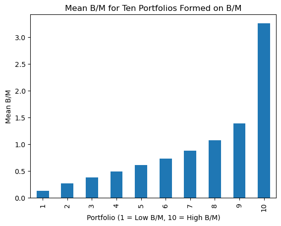
Returns from July of year \(t\) to June of year \(t+1\)
Now we assign returns to each of these ten portfolios.
returns = (
    pd.merge_asof(
        left=crsp.sort_values(by=['date', 'PERMNO']),
        right=portfolios.sort_values(by=['Date', 'PERMNO']),
        left_on='date',
        right_on='Date',
        by='PERMNO',
        tolerance=pd.Timedelta('366 days')
    )
    [['PERMNO', 'date', 'RET', 'Portfolio']]
    .dropna()
    .assign(Portfolio=lambda x: x['Portfolio'].astype(int))
    .rename(columns={'date': 'Date'})
)returns| PERMNO | Date | RET | Portfolio | |
|---|---|---|---|---|
| 37636 | 10006 | 1966-07-31 | -0.0149 | 6 |
| 37640 | 10102 | 1966-07-31 | -0.0545 | 6 |
| 37641 | 10137 | 1966-07-31 | 0.0105 | 4 |
| 37642 | 10145 | 1966-07-31 | -0.0129 | 6 |
| 37643 | 10153 | 1966-07-31 | -0.0788 | 9 |
| ... | ... | ... | ... | ... |
| 3457680 | 93397 | 2024-12-31 | -0.1174 | 5 |
| 3457681 | 93426 | 2024-12-31 | 0.0218 | 7 |
| 3457682 | 93429 | 2024-12-31 | -0.0947 | 3 |
| 3457683 | 93434 | 2024-12-31 | 0.1333 | 10 |
| 3457684 | 93436 | 2024-12-31 | 0.1700 | 1 |
2690626 rows × 4 columns
Performance of Portfolios Formed on B/M
(
    returns
    .groupby(['Portfolio', 'Date'])
    ['RET']
    .mean()
    .groupby(['Portfolio'])
    .mean()
    .mul(100)
    .plot(kind='bar')
)
plt.ylabel('Mean Monthly Return (%)')
plt.xlabel('Portfolio (1 = Low B/M, 10 = High B/M)')
plt.title('Mean Monthly Returns for Equal-Weighted Portfolios Formed on B/M')
plt.show()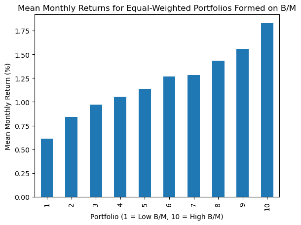
(
    returns
    .groupby(['Portfolio', 'Date'])
    ['RET']
    .mean()
    .unstack('Portfolio')
    .add(1)
    .cumprod()
    .plot()
)
plt.semilogy()
plt.ylabel('Value of $1 Investment')
plt.title('Values of $1 Investments in Equal-Weighted Portfolios Formed on B/M')
plt.show()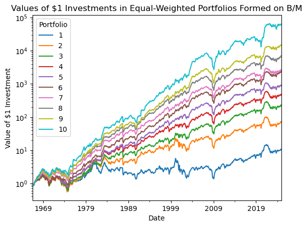
(
    returns
    .groupby(['Portfolio', 'Date'])
    ['RET']
    .mean()
    .unstack('Portfolio')
    .assign(Diff=lambda x: x[10] - x[1])
    ['Diff']
    .rolling(12*10)
    .mean()
    .mul(100)
    .plot()
)
plt.ylabel('10-year Rolling Mean of Monthly Spread (%)')
plt.title('10-year Rolling Mean of Monthly Spread\n Between Value and Growth Portfolios')
plt.show()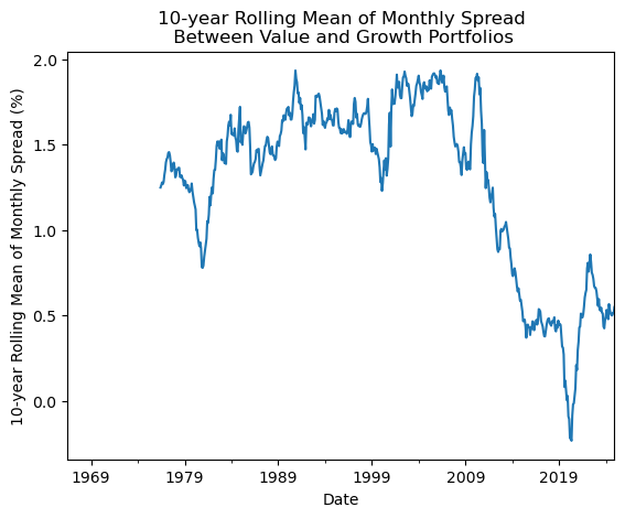
References
Fama, Eugene F., and Kenneth R. French. 1993. “Common Risk Factors in the Returns on Stocks and Bonds.” Journal of Financial Economics 33 (1): 3–56.
Gray, Wesley R., and Tobias E. Carlisle. 2012. Quantitative Value: A Practitioner’s Guide to Automating Intelligent Investment and Eliminating Behavioral Errors. John Wiley & Sons.