import matplotlib.pyplot as plt
import numpy as np
import pandas as pd
import pandas_datareader as pdr
import seaborn as sns
import statsmodels.api as sm
import yfinance as yfHerron Topic 2 - Practice - Sec 04
FINA 6333 for Spring 2025
%precision 4
pd.options.display.float_format = '{:.4f}'.format
# %config InlineBackend.figure_format = 'retina'
Announcements
- I am still grading your projects; I hope to finish them by next Tuesday
- I posted 50 practice problems to prepare for the end-of-course Programming Assessment here: https://northeastern.instructure.com/courses/207607/discussion_topics/2727917
- I built 5 autograded notebooks to help you prepare for the assessment, and I will build more in the coming weeks
- To run these notebooks, install the
otter-graderpackage: In the Anaconda command prompt (or Terminal on Mac) runconda activate fina6333thenconda install otter-grader - See the video at the link above for details
Five-Minute Review
- Technical analysis (TA) is a method of evaluating trends in trading prices and volume (and open interest in the futures and options markets only)
- The three tenants of TA are:
- Markets discount everything
- Prices move in trends
- History repeats itself, so these trends are recurring
- Academics have not found much evidence that TA generate profits that exceed transaction costs, but we will spend a week on it for three reasons:
- You asked for it, and it will help build our data analytics skills
- It is a small part of the Chartered Financial Analyst (CFA) curriculum
- That TA still receives attention 60 years after the Efficient Markets Hypothesis (EMH) suggests that it has some value that academics have been unable to measure
Practice
Implement the SMA(20) strategy with BTC-USD from the lecture notebook
Try to create the btc_sma data frame from the btc data frame in one code cell with one assignment (i.e., one =).
btc = (
    yf.download(
        tickers='BTC-USD',
        auto_adjust=False,
        progress=False,
        multi_level_index=False
    )
    .iloc[:-1] # drop incomplete trading day
)
After class, I converted our code to a function. We might want to test different moving average parameters, and a function makes these tests easier.
The following calc_sma() function accepts:
- A data frame
dfof daily values fromyfinance.download() - An integer
windowthat specifies the number of trading days in the SMA window
And returns the original data frame df plus the following columns:
Returnwith daily returnsSMAfor thewindow-trading-day moving averagePositionfor the weight on the security each dayStrategyfor the return on the strategy each day
def calc_sma(df, window=20):
    return (
        df
        .assign(
            Return=lambda x: x['Adj Close'].pct_change(),
            SMA=lambda x: x['Adj Close'].rolling(window=window).mean(),
            Position=lambda x: np.select(
                condlist=[
                    x['Adj Close'].shift(1) > x['SMA'].shift(1),
                    x['Adj Close'].shift(1) <= x['SMA'].shift(1)
                ],
                choicelist=[1, 0],
                default=np.nan
            ),
            Strategy=lambda x: x['Position'] * x['Return']
        )
    )
btc_sma = btc.pipe(calc_sma, window=20)It can be helpful to visualize a few places where the price (here Adj Close) crosses the moving average (here SMA(20)). In class, we found that there are a few changes in position in the middle of October, 2014. The following code create two subplots in one figure, then puts one plot in each of the subplots.
For the first crossover on October 12, we buy at the close on October 12 and earn the security return on October 13. For the second crossover on October 23, we sell at the close on October 23 and earn zero return on October 24.
columns_sma20 = {
    'Adj Close': 'Price',
    'SMA': 'SMA(20)',
    'Return': 'Buy-And-Hold',
    'Strategy': 'SMA(20)'
}
fig, ax = plt.subplots(2, 1)
df = btc_sma.loc['2014-10-10':'2014-10-25']
df[['Adj Close', 'SMA']].rename(columns=columns_sma20).plot(ax=ax[0])
df[['Position']].plot(ax=ax[1])
plt.suptitle('SMA(20) Crossovers and Positions in Mid-October 2014')
plt.tight_layout()
plt.show()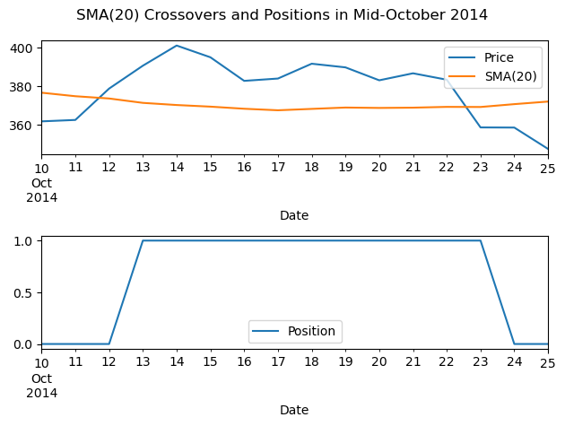
We can compare the total returns on BTC-USD and our SMA(20) strategy! We .dropna() first because the SMA(20) strategy needs 20 days of data to make its first investing decision.
(
    btc_sma
    [['Return', 'Strategy']]
    .dropna()
    .rename(columns=columns_sma20)
    .add(1)
    .cumprod()
    .plot()
)
plt.semilogy()
plt.suptitle('Comparison of One-Dollar Investments in BTC-USD Strategies')
plt.ylabel('Value of One-Dollar Investments')
plt.show()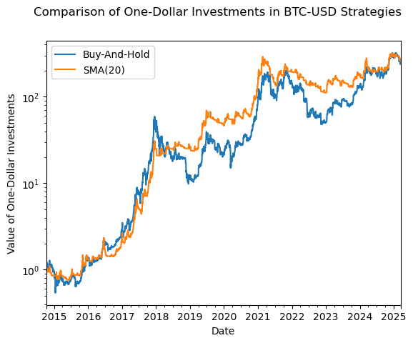
These total returns, at least today, are similar!
(
    btc_sma
    [['Return', 'Strategy']]
    .dropna()
    .rename(columns=columns_sma20)
    .add(1)
    .prod()
    .plot(kind='bar')
)
plt.suptitle('Comparison of One-Dollar Investments in BTC-USD Strategies')
plt.ylabel('Value of One-Dollar Investments')
plt.show()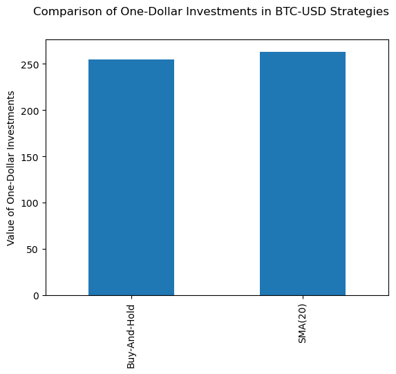
However, the Sharpe ratio of the SMA(20) is higher, because time out of the market when Position=0 reduces risk. For simplicity, we will ignore the risk-free rate in the Sharpe ratio formula.
(
    btc_sma
    [['Return', 'Strategy']]
    .dropna()
    .rename(columns=columns_sma20)
    .apply(lambda x: np.sqrt(252) * x.mean() / x.std())
    .plot(kind='bar')
)
plt.suptitle('Comparison of Reward-to-Risk in BTC-USD Strategies')
plt.ylabel('Sharpe Ratio')
plt.show()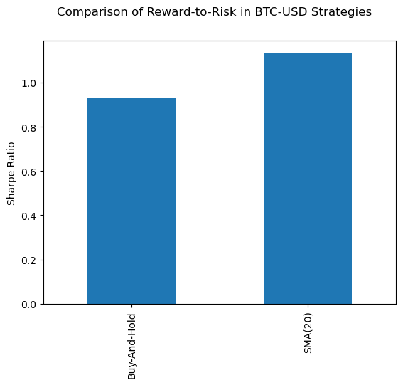
But how persistent is this outperformance in terms of reward-to-risk ratios? We can quickly modify the code above to calculate Sharpe ratios each year! We find that SMA(20) Sharpe ratio edge is not persistent.
df = (
    btc_sma
    [['Return', 'Strategy']]
    .dropna()
    .rename(columns=columns_sma20)
    .resample('YE')
    .apply(lambda x: np.sqrt(252) * x.mean() / x.std())
)
df.index = df.index.year
df.plot(kind='bar')
plt.suptitle('Comparison of Reward-to-Risk in BTC-USD Strategies over Time')
plt.ylabel('Sharpe Ratio')
plt.show()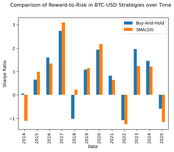
We can use our list comprehension skills to easily try several window sizes!
def CAGR(x):
    T = x.count()
    return (x.add(1).prod() ** (252 / T)) - 1
def Sharpe(x, ann_fac=np.sqrt(252)):
return ann_fac * x.mean() / x.std()columns_sman = {
'Adj Close': 'Price',
'SMA': 'SMA(N)',
'Return': 'Buy-And-Hold',
'Strategy': 'SMA(N)'
}windows = list(range(5, 55, 5))
btc_smas = (
pd.concat(
objs=[
btc.pipe(calc_sma, window=w)[['Return', 'Strategy']].agg([CAGR, Sharpe])
for w in windows
],
keys=windows,
names=['Window', 'Statistic']
)
.rename(columns=columns_sman)
) btc_smas| Buy-And-Hold | SMA(N) | ||
|---|---|---|---|
| Window | Statistic | ||
| 5 | CAGR | 0.4090 | 0.5002 |
| Sharpe | 0.8877 | 1.2139 | |
| 10 | CAGR | 0.4090 | 0.4558 |
| Sharpe | 0.8877 | 1.1490 | |
| 15 | CAGR | 0.4090 | 0.4687 |
| Sharpe | 0.8877 | 1.1826 | |
| 20 | CAGR | 0.4090 | 0.4454 |
| Sharpe | 0.8877 | 1.1327 | |
| 25 | CAGR | 0.4090 | 0.4756 |
| Sharpe | 0.8877 | 1.1728 | |
| 30 | CAGR | 0.4090 | 0.4656 |
| Sharpe | 0.8877 | 1.1521 | |
| 35 | CAGR | 0.4090 | 0.5298 |
| Sharpe | 0.8877 | 1.2464 | |
| 40 | CAGR | 0.4090 | 0.5818 |
| Sharpe | 0.8877 | 1.3250 | |
| 45 | CAGR | 0.4090 | 0.5621 |
| Sharpe | 0.8877 | 1.2892 | |
| 50 | CAGR | 0.4090 | 0.5258 |
| Sharpe | 0.8877 | 1.2250 |
(
    btc_smas
    .reset_index()
    .melt(
        id_vars=['Window', 'Statistic'],
        value_vars=['Buy-And-Hold', 'SMA(N)'],
        var_name='Strategy',
        value_name='Value'
    )
    .pipe(
        sns.catplot,
        x='Window',
        col='Statistic',
        hue='Strategy',
        y='Value',
        kind='bar',
        sharey=False
    )
)
plt.suptitle('Comparsion of BTC-USD Buy-And-Hold and SMA(N) for Various Ns', y=1.05)
plt.show()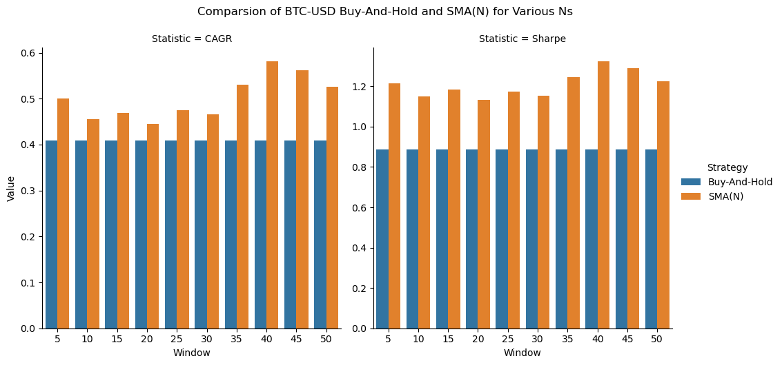
Investigate how SMA(20) generates returns
Consider the following:
- Does SMA(20) avoid the worst performing days? How many of the worst 20 days does SMA(20) avoid? Try the
.nlargest()method. - Does SMA(20) preferentially avoid low-return days? Try to combine the
.groupby()method andpd.qcut()function. - Does SMA(20) preferentially avoid high-volatility days? Try to combine the
.groupby()method andpd.qcut()function.
The SMA(20) does well here because it avoids 17 of the 20 worst days, without avoiding the best days.
btc_sma.loc[btc_sma['Return'].nsmallest(20).index, ['Position']].value_counts()Position
0.0000 17
1.0000 3
Name: count, dtype: int64btc_sma.loc[btc_sma['Return'].nlargest(20).index, ['Position']].value_counts()Position
0.0000 10
1.0000 10
Name: count, dtype: int64We can also look at the descriptive statistics by Postiion and strategy. Two observations:
- The
mincolumn shows that SMA(20) misses the bad days, like we see above - The
meaninPosition=1is about 5 times higher than inPosition=0
(
    btc_sma
    [['Position', 'Return', 'Strategy']]
    .dropna()
    .groupby('Position')
    .describe()
    .rename(columns=columns_sma20)
    .rename_axis(columns=['Strategy', 'Statistic'])
    .stack('Strategy', future_stack=True)
)| Statistic | count | mean | std | min | 25% | 50% | 75% | max | |
|---|---|---|---|---|---|---|---|---|---|
| Position | Strategy | ||||||||
| 0.0000 | Buy-And-Hold | 1721.0000 | 0.0008 | 0.0390 | -0.3717 | -0.0138 | 0.0012 | 0.0162 | 0.2394 |
| SMA(20) | 1721.0000 | 0.0000 | 0.0000 | 0.0000 | 0.0000 | 0.0000 | 0.0000 | 0.0000 | |
| 1.0000 | Buy-And-Hold | 2091.0000 | 0.0032 | 0.0333 | -0.1409 | -0.0114 | 0.0013 | 0.0173 | 0.2525 |
| SMA(20) | 2091.0000 | 0.0032 | 0.0333 | -0.1409 | -0.0114 | 0.0013 | 0.0173 | 0.2525 |
We can also use the seaborn package to visualize Position (i.e., the portfolio weight on Bitcoin) during periods of high and low Bitcoin returns and volatility. The SMA(20) strategy is long Bitcoin about 55% of the time, whether Bitcoin returns are high (bin 2) or low (bin 1).
(
    btc_sma
    [['Return', 'Position']]
    .dropna()
    .assign(Return_Bin=lambda x: pd.qcut(x['Return'], q=3))
    .pipe(
        sns.barplot,
        x='Return_Bin',
        y='Position'
    )
)

plt.title('Fraction of Time SMA(20) Strategy is Long by Return Bin')
plt.show()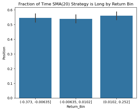
However, the SMA(20) stateegy, for this security, sample, and window, spends less times in Bitcoind during volatilit times.
(
    btc_sma
    [['Return', 'Position']]
    .dropna()
    .assign(Volatility_Bin=lambda x: pd.qcut(x['Return'].rolling(20).std(), q=3))
    .pipe(
        sns.barplot,
        x='Volatility_Bin',
        y='Position'
    )
)

plt.title('Fraction of Time SMA(20) Strategy is Long by Volatility Bin')
plt.show()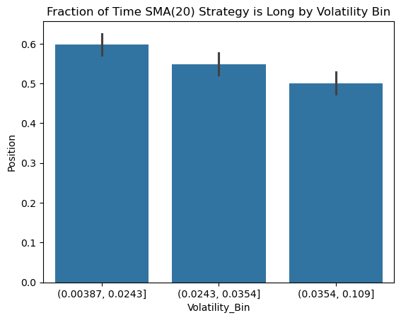
Implement the SMA(20) strategy with IBM
How often does SMA(20) outperform buy-and-hold with 10-year rolling windows?
ibm = (
    yf.download(
        tickers='IBM',
        auto_adjust=False,
        progress=False,
        multi_level_index=False
    )
    .iloc[:-1] # drop incomplete trading day
)
ibm_sma = ibm.pipe(calc_sma, window=20)(
ibm_sma
[['Return', 'Strategy']]
.dropna()
.rename(columns=columns_sma20)
.add(1)
.cumprod()
.plot()
)
plt.semilogy()
plt.suptitle('Comparison of One-Dollar Investments in IBM Strategies')
plt.ylabel('Value of One-Dollar Investments')
plt.show()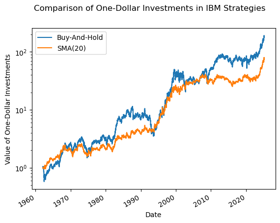
Over the full, 60-year sample, SMA(20) underperforms buy-and-hold. What about on rolling ten-year windows? The results look balanced, and neither clearly outperforms.
(
    ibm_sma
    [['Return', 'Strategy']]
    .dropna()
    .rename(columns=columns_sma20)
    .pipe(np.log1p)
    .rolling(window=10*252)
    .sum()
    .pipe(np.exp)
    .plot()
)
plt.semilogy()
plt.suptitle('Comparison of One-Dollar Investments in IBM Strategies')
plt.ylabel('Value of One-Dollar Investments')
plt.show()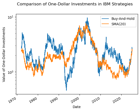
We can quantify how often SMA(20) outperform buy-and-hold. SMA(20) outperforms only 24% of the time!
(
    ibm_sma
    [['Return', 'Strategy']]
    .dropna()
    .pipe(np.log1p)
    .rolling(window=10*252)
    .sum()
    .pipe(np.exp)
    .pipe(lambda x: x['Strategy'] > x['Return'])
    .mean()
)0.2378windows = list(range(5, 55, 5))
ibm_smas = (
pd.concat(
objs=[
ibm.pipe(calc_sma, window=w)[['Return', 'Strategy']].agg([CAGR, Sharpe])
for w in windows
],
keys=windows,
names=['Window', 'Statistic']
)
.rename(columns=columns_sman)
) (
ibm_smas
.reset_index()
.melt(
id_vars=['Window', 'Statistic'],
value_vars=['Buy-And-Hold', 'SMA(N)'],
var_name='Strategy',
value_name='Value'
)
.pipe(
sns.catplot,
x='Window',
col='Statistic',
hue='Strategy',
y='Value',
kind='bar',
sharey=False
)
)
plt.suptitle('Comparsion of IBM Buy-And-Hold and SMA(N) for Various Ns', y=1.05)
plt.show()
Implement a long-only BB(20, 2) strategy with Bitcoin
Bollinger Bands are bands around a trend, typically defined in terms of simple moving averages and volatilities. A long-only BB(20, 2) strategy has upper and lower bands at 2 standard deviations above and below the SMA(20). It invests as follows:
- Buy when the closing price crosses LB(20) from below
- Sell when the closing price crosses UB(20) from above
- No short-selling
The long-only BB(20, 2) is more difficult to implement than the long-only SMA(20) because we need to track buys and sells. For example, if the closing price is between LB(20) and BB(20), we need to know if our last trade was a buy or a sell. Further, if the closing price is below LB(20), we can still be long because we sell when the closing price crosses UB(20) from above.
More on Bollinger Bands here and here.
def calc_bb(df, m=20, n=2):
    return (
        df
        .assign(
            Return=lambda x: x['Adj Close'].pct_change(),
            SMA=lambda x: x['Adj Close'].rolling(window=m).mean(),
            SMV=lambda x: x['Adj Close'].rolling(window=m).std(),
            UB=lambda x: x['SMA'] + n*x['SMV'],
            LB=lambda x: x['SMA'] - n*x['SMV'],
            Position_w_nan=lambda x: np.select(
                condlist=[
                    (x['Adj Close'].shift(1) > x['LB'].shift(1)) & (x['Adj Close'].shift(2) <= x['LB'].shift(2)),
                    (x['Adj Close'].shift(1) < x['UB'].shift(1)) & (x['Adj Close'].shift(2) >= x['UB'].shift(2))
                ],
                choicelist=[1, 0],
                default=np.nan
            ),
            Position=lambda x: x['Position_w_nan'].ffill(),
            Strategy=lambda x: x['Position'] * x['Return']
        )
    )
btc_bb = btc.pipe(calc_bb)The BB(20, 2) only spends 40% of its time long BTC!
btc_bb['Position'].mean()0.4013And BTC-USD performance is worse when it long that when its neutral!
- Mean daily return is lower
- Volatility of daily returns is higher
- Every percentile of the distribution is worse
btc_bb.groupby('Position')['Return'].describe()| count | mean | std | min | 25% | 50% | 75% | max | |
|---|---|---|---|---|---|---|---|---|
| Position | ||||||||
| 0.0000 | 2268.0000 | 0.0027 | 0.0343 | -0.1874 | -0.0110 | 0.0019 | 0.0172 | 0.2525 |
| 1.0000 | 1520.0000 | 0.0013 | 0.0386 | -0.3717 | -0.0149 | 0.0007 | 0.0161 | 0.2394 |
columns_bb = {
    'Adj Close': 'Price',
    'Return': 'Buy-And-Hold',
    'Strategy': 'BB(20, 2)'
}
(
btc_bb
[['Return', 'Strategy']]
.dropna()
.rename(columns=columns_bb)
.add(1)
.cumprod()
.plot()
)
plt.semilogy()
plt.suptitle('Comparison of One-Dollar Investments in BTC-USD Strategies')
plt.ylabel('Value of One-Dollar Investments')
plt.show()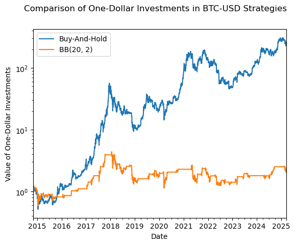
Here are the final values of $1 investments, which are difficult to read on the log scale above.
(
    btc_bb
    [['Return', 'Strategy']]
    .rename(columns=columns_bb)
    .add(1)
    .prod()
    .rename_axis('Strategy')
    .to_frame('Value of One-Dollar Investment')
)| Value of One-Dollar Investment | |
|---|---|
| Strategy | |
| Buy-And-Hold | 183.6056 |
| BB(20, 2) | 2.1877 |
We need a more complex plot to better understand what is going on!
import matplotlib.ticker as tickerfig, ax = plt.subplots(nrows=2, ncols=1, sharex=True)
df = btc_bb.loc['2017-09':'2017-12']
ax[0].plot(df[['Adj Close']], label='Price')
ax[0].plot(df[['SMA']], label='SMA(20)')
ax[0].plot(df[['UB']], label='LB and UB', color='green', linestyle=':')
ax[0].plot(df[['LB']], color='green', linestyle=':')
ax[0].legend()
ax[0].set_ylabel('Price ($)')
ax[1].plot(df[['Position']], label='Signal')
ax[1].legend()
ax[1].set_ylabel('Position')
ax[0].yaxis.set_major_formatter(ticker.StrMethodFormatter('{x:,.0f}'))
fig.autofmt_xdate()
plt.suptitle('Key Variables in BTC-USD BB(20, 2) Strategy')
plt.show()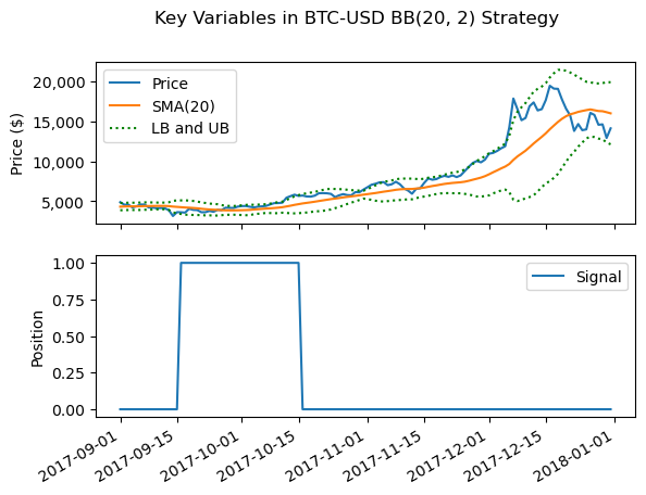
Implement a long-short RSI(14) strategy with Bitcoin
From Fidelity:
The Relative Strength Index (RSI), developed by J. Welles Wilder, is a momentum oscillator that measures the speed and change of price movements. The RSI oscillates between zero and 100. Traditionally the RSI is considered overbought when above 70 and oversold when below 30. Signals can be generated by looking for divergences and failure swings. RSI can also be used to identify the general trend.
The RSI formula: \(RSI(n) = 100 - \frac{100}{1 + RS(n)}\), where \(RS(n) = \frac{SMA(U, n)}{SMA(D, n)}\). For “up days”, \(U = \Delta \text{Adj\ Close}\) and \(D = 0\). For “down days”, \(U = 0\) and \(D = - \Delta \text{Adj\ Close}\).
We will implement a long-short RSI(14) as follows:
- Buy when the RSI crosses 30 from below, and sell when the RSI crosses 50 from below
- Short when the RSI crosses 70 from above, and cover when the RSI crosses 50 from above
More about RSI here.
def calc_rsi(df, window=14, lo=30, mid=50, hi=70):
    return (
        df
        .assign(
            Return=lambda x: x['Adj Close'].pct_change(),
            # This approach with .max() and .min() handles NA values better than the in-class solution
            Diff=lambda x: x['Adj Close'].diff(),
            Zero=0,
            U=lambda x: x[['Diff', 'Zero']].max(axis=1, skipna=False),
            D=lambda x: -x[['Diff', 'Zero']].min(axis=1, skipna=False),
            SMAU=lambda x: x['U'].rolling(window=window).mean(),
            SMAD=lambda x: x['D'].rolling(window=window).mean(),
            RS=lambda x: x['SMAU'] / x['SMAD'],
            RSI=lambda x: 100 - 100 / (1 + x['RS']),
            Position_w_nan=lambda x: np.select(
                condlist=[
                    (x['RSI'].shift(1) > lo) & (x['RSI'].shift(2) <= lo),
                    (x['RSI'].shift(1) > mid) & (x['RSI'].shift(2) <= mid),
                    (x['RSI'].shift(1) < hi) & (x['RSI'].shift(2) >= hi),
                    (x['RSI'].shift(1) < mid) & (x['RSI'].shift(2) >= mid),
                ],
                choicelist=[1, 0, -1, 0],
                default=np.nan
            ),
            Position=lambda x: x['Position_w_nan'].ffill(),
            Strategy=lambda x: x['Position'] * x['Return']
        )
    )
btc_rsi = btc.pipe(calc_rsi)columns_rsi = {
'Adj Close': 'Price',
'Return': 'Buy-And-Hold',
'Strategy': 'RSI(14)'
}(
btc_rsi
[['Return', 'Strategy']]
.dropna()
.rename(columns=columns_rsi)
.add(1)
.cumprod()
.plot()
)
plt.semilogy()
plt.suptitle('Comparison of One-Dollar Investments in BTC-USD Strategies')
plt.ylabel('Value of One-Dollar Investments')
plt.show()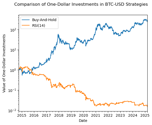
Implement a golden cross with Bitcoin
Someone in Section 04 mentioned two-moving average strategies, so I added this golden cross, where the 50-day SMA crosses the 200-day SMA, to every section.
From Grok:
In technical analysis, a golden cross is a bullish chart pattern that occurs when a short-term moving average (typically the 50-day moving average) crosses above a long-term moving average (typically the 200-day moving average). This crossover is considered a signal that a stock, index, or other asset may be entering a sustained upward trend, suggesting potential buying opportunities for traders and investors.
More here.
def calc_cross(df, long=200, short=50):
    return (
        df
        .assign(
            Return=lambda x: x['Adj Close'].pct_change(),
            SMAL=lambda x: x['Adj Close'].rolling(window=long).mean(),
            SMAS=lambda x: x['Adj Close'].rolling(window=short).mean(),
            Position=lambda x: np.select(
                condlist=[
                    x['SMAS'].shift(1) > x['SMAL'].shift(1),
                    x['SMAS'].shift(1) <= x['SMAL'].shift(1)
                ],
                choicelist=[1, 0],
                default=np.nan
            ),
            Strategy=lambda x: x['Position'] * x['Return']
        )
    )
btc_cross = btc.pipe(calc_cross, long=200, short=50)columns_cross = {
'Adj Close': 'Price',
'SMAL': 'SMA(200)',
'SMAS': 'SMA(50)',
'Return': 'Buy-And-Hold',
'Strategy': 'Golden Cross(200, 50)'
}btc_cross.query('Position == 1')| Adj Close | Close | High | Low | Open | Volume | Return | SMAL | SMAS | Position | Strategy | |
|---|---|---|---|---|---|---|---|---|---|---|---|
| Date | |||||||||||
| 2015-07-15 | 285.8290 | 285.8290 | 293.2480 | 285.3670 | 288.0450 | 27486600 | -0.0057 | 247.7823 | 249.0083 | 1.0000 | -0.0057 |
| 2015-07-16 | 278.0890 | 278.0890 | 291.1830 | 275.2400 | 286.0420 | 49482600 | -0.0271 | 247.5865 | 249.8244 | 1.0000 | -0.0271 |
| 2015-07-17 | 279.4720 | 279.4720 | 280.2800 | 272.0430 | 278.0910 | 27591400 | 0.0050 | 247.4205 | 250.6657 | 1.0000 | 0.0050 |
| 2015-07-18 | 274.9010 | 274.9010 | 282.5270 | 274.0750 | 279.3310 | 25187100 | -0.0164 | 247.2414 | 251.4218 | 1.0000 | -0.0164 |
| 2015-07-19 | 273.6140 | 273.6140 | 275.6700 | 272.5130 | 274.7670 | 15332500 | -0.0047 | 247.0085 | 252.2272 | 1.0000 | -0.0047 |
| ... | ... | ... | ... | ... | ... | ... | ... | ... | ... | ... | ... |
| 2025-03-10 | 78532.0000 | 78532.0000 | 83955.9297 | 77420.5938 | 80597.1484 | 54061099422 | -0.0257 | 83357.9603 | 95531.6020 | 1.0000 | -0.0257 |
| 2025-03-11 | 82862.2109 | 82862.2109 | 83577.7578 | 76624.2500 | 78523.8750 | 54702837196 | 0.0551 | 83451.7996 | 95148.5130 | 1.0000 | 0.0551 |
| 2025-03-12 | 83722.3594 | 83722.3594 | 84358.5781 | 80635.2500 | 82857.3750 | 40353484454 | 0.0104 | 83549.5164 | 94700.0348 | 1.0000 | 0.0104 |
| 2025-03-13 | 81066.7031 | 81066.7031 | 84301.6953 | 79931.8516 | 83724.9219 | 31412940153 | -0.0317 | 83633.1822 | 94248.3075 | 1.0000 | -0.0317 |
| 2025-03-14 | 83969.1016 | 83969.1016 | 85263.2891 | 80797.5625 | 81066.9922 | 29588112414 | 0.0358 | 83738.6244 | 93848.4861 | 1.0000 | 0.0358 |
2320 rows × 11 columns
fig, ax = plt.subplots(2, 1)
df = btc_cross.loc['2015-07':'2015-12']
df[['Adj Close', 'SMAL', 'SMAS']].rename(columns=columns_cross).plot(ax=ax[0])
df[['Position']].plot(ax=ax[1])
plt.suptitle('Golden Cross(200, 50) Crossovers and Positions in 2015H2')
plt.tight_layout()
plt.show()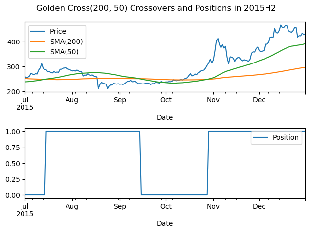
(
    btc_cross
    [['Return', 'Strategy']]
    .dropna()
    .rename(columns=columns_cross)
    .add(1)
    .cumprod()
    .plot()
)
plt.semilogy()
plt.suptitle('Comparison of One-Dollar Investments in BTC-USD Strategies')
plt.ylabel('Value of One-Dollar Investments')
plt.show()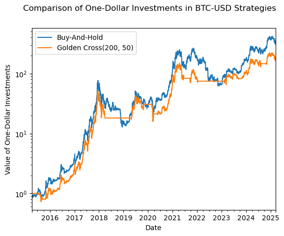
Compare all strategies
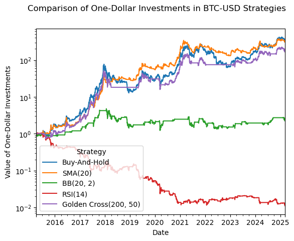
I added this comparison of all strategies after class.
df = (
    btc_sma[['Return', 'Strategy']]
    .join(btc_bb[['Strategy']], rsuffix='_bb')
    .join(btc_rsi[['Strategy']], rsuffix='_rsi')
    .join(btc_cross[['Strategy']], rsuffix='_cross')
    .dropna()
)


(
    df
    .add(1)
    .cumprod()
    .rename_axis(columns='Strategy')
    .rename(columns={
        'Return': 'Buy-And-Hold',
        'Strategy': 'SMA(20)',
        'Strategy_bb': 'BB(20, 2)',
        'Strategy_rsi': 'RSI(14)',
        'Strategy_cross': 'Golden Cross(200, 50)',
    })
    .plot()
)

plt.semilogy()
plt.suptitle('Comparison of One-Dollar Investments in BTC-USD Strategies')
plt.ylabel('Value of One-Dollar Investments')
plt.show()