import matplotlib.pyplot as plt
import numpy as np
import pandas as pd
import pandas_datareader as pdr
import yfinance as yfMcKinney Chapter 11 - Time Series
FINA 6333 for Spring 2025
%precision 4
pd.options.display.float_format = '{:.4f}'.format
# %config InlineBackend.figure_format = 'retina'
Introduction
Chapter 11 of McKinney (2022) discusses time series and panel data, which is where pandas excels! We will use these time series and panel tools every day for the rest of the course.
We will focus on:
- Slicing a data frame or series by date or date range
- Using
.shift()to create leads and lags of variables - Using
.resample()to change the frequency of variables - Using
.rolling()to aggregate data over moving or rolling windows
Note: Indented block quotes are from McKinney (2022) unless otherwise indicated. The section numbers here differ from McKinney (2022) because we will only discuss some topics.
Time Series Basics
Let us create a time series to play with.
from datetime import datetime
dates = [
    datetime(2011, 1, 2),
    datetime(2011, 1, 5),
    datetime(2011, 1, 7),
    datetime(2011, 1, 8),
    datetime(2011, 1, 10),
    datetime(2011, 1, 12)
]
np.random.seed(42)
ts = pd.Series(np.random.randn(6), index=dates)

ts
2011-01-02 0.4967
2011-01-05 -0.1383
2011-01-07 0.6477
2011-01-08 1.5230
2011-01-10 -0.2342
2011-01-12 -0.2341
dtype: float64Note that pandas converts the datetime objects to a pandas DatetimeIndex object and a single index value is a Timestamp object.
ts.indexDatetimeIndex(['2011-01-02', '2011-01-05', '2011-01-07', '2011-01-08',
'2011-01-10', '2011-01-12'],
dtype='datetime64[ns]', freq=None)ts.index[0]Timestamp('2011-01-02 00:00:00')Recall that pandas automatically aligns objects on indexes.
ts2011-01-02 0.4967
2011-01-05 -0.1383
2011-01-07 0.6477
2011-01-08 1.5230
2011-01-10 -0.2342
2011-01-12 -0.2341
dtype: float64ts.iloc[::2]2011-01-02 0.4967
2011-01-07 0.6477
2011-01-10 -0.2342
dtype: float64ts + ts.iloc[::2]2011-01-02 0.9934
2011-01-05 NaN
2011-01-07 1.2954
2011-01-08 NaN
2011-01-10 -0.4683
2011-01-12 NaN
dtype: float64If we want to assign a default for missing values on the fly, we can use the .add() method.
ts.add(ts.iloc[::2], fill_value=1_000_000)2011-01-02 0.9934
2011-01-05 999999.8617
2011-01-07 1.2954
2011-01-08 1000001.5230
2011-01-10 -0.4683
2011-01-12 999999.7659
dtype: float64Indexing, Selection, Subsetting
pandas uses U.S.-style date strings (e.g., “M/D/Y”) or unambiguous date strings (e.g., “YYYY-MM-DD”) to select data.
ts.loc['1/10/2011'] # M/D/YYYY-0.2342ts.loc['2011-01-10'] # YYYY-MM-DD-0.2342ts.loc['20110110'] # YYYYMMDD-0.2342ts.loc['10-Jan-2011'] # D-Mon-YYYY-0.2342ts.loc['Jan-10-2011'] # Mon-D-YYYY-0.2342pandas does not use U.K.-style date strings.
# ts.loc['10/1/2011'] # D/M/YYYY # KeyError: '10/1/2011'Let us create a longer time series to play with.
np.random.seed(42)
longer_ts = pd.Series(
    data=np.random.randn(1000),
    index=pd.date_range('1/1/2000', periods=1000)
)longer_ts2000-01-01 0.4967
2000-01-02 -0.1383
2000-01-03 0.6477
2000-01-04 1.5230
2000-01-05 -0.2342
...
2002-09-22 -0.2811
2002-09-23 1.7977
2002-09-24 0.6408
2002-09-25 -0.5712
2002-09-26 0.5726
Freq: D, Length: 1000, dtype: float64We can specify a year-month to slice all of the observations in May of 2001.
longer_ts.loc['2001-05']2001-05-01 -0.6466
2001-05-02 -1.0815
2001-05-03 1.6871
2001-05-04 0.8816
2001-05-05 -0.0080
2001-05-06 1.4799
2001-05-07 0.0774
2001-05-08 -0.8613
2001-05-09 1.5231
2001-05-10 0.5389
2001-05-11 -1.0372
2001-05-12 -0.1903
2001-05-13 -0.8756
2001-05-14 -1.3828
2001-05-15 0.9262
2001-05-16 1.9094
2001-05-17 -1.3986
2001-05-18 0.5630
2001-05-19 -0.6506
2001-05-20 -0.4871
2001-05-21 -0.5924
2001-05-22 -0.8640
2001-05-23 0.0485
2001-05-24 -0.8310
2001-05-25 0.2705
2001-05-26 -0.0502
2001-05-27 -0.2389
2001-05-28 -0.9076
2001-05-29 -0.5768
2001-05-30 0.7554
2001-05-31 0.5009
Freq: D, dtype: float64We can also specify a year to slice all observations in 2001.
longer_ts.loc['2001']2001-01-01 0.2241
2001-01-02 0.0126
2001-01-03 0.0977
2001-01-04 -0.7730
2001-01-05 0.0245
...
2001-12-27 0.0184
2001-12-28 0.3476
2001-12-29 -0.5398
2001-12-30 -0.7783
2001-12-31 0.1958
Freq: D, Length: 365, dtype: float64If we sort our data chronologically, we can also slice with a range of date strings.
ts.loc['1/6/2011':'1/10/2011']2011-01-07 0.6477
2011-01-08 1.5230
2011-01-10 -0.2342
dtype: float64However, we cannot date slice if our data are not sorted chronologically.
ts2 = ts.sort_values()ts22011-01-10 -0.2342
2011-01-12 -0.2341
2011-01-05 -0.1383
2011-01-02 0.4967
2011-01-07 0.6477
2011-01-08 1.5230
dtype: float64The following date slice fails because ts2 is not sorted chronologically.
# ts2.loc['1/6/2011':'1/11/2011'] # KeyError: 'Value based partial slicing on non-monotonic DatetimeIndexes with non-existing keys is not allowed.'We can use the .sort_index() method first to allow date slices.
ts2.sort_index()['1/6/2011':'1/11/2011']2011-01-07 0.6477
2011-01-08 1.5230
2011-01-10 -0.2342
dtype: float64As with label slices, date slices are inclusive on both ends.
longer_ts.loc['1/6/2001':'1/11/2001']2001-01-06 0.4980
2001-01-07 1.4511
2001-01-08 0.9593
2001-01-09 2.1532
2001-01-10 -0.7673
2001-01-11 0.8723
Freq: D, dtype: float64Recall that if we modify a slice, we modify the original series or data frame.
Remember that slicing in this manner produces views on the source time series like slicing NumPy arrays. This means that no data is copied and modifications on the slice will be reflected in the original data.
ts3 = ts.copy()ts32011-01-02 0.4967
2011-01-05 -0.1383
2011-01-07 0.6477
2011-01-08 1.5230
2011-01-10 -0.2342
2011-01-12 -0.2341
dtype: float64ts4 = ts3.iloc[:3]ts42011-01-02 0.4967
2011-01-05 -0.1383
2011-01-07 0.6477
dtype: float64ts4.iloc[:] = 2001ts42011-01-02 2001.0000
2011-01-05 2001.0000
2011-01-07 2001.0000
dtype: float64ts32011-01-02 2001.0000
2011-01-05 2001.0000
2011-01-07 2001.0000
2011-01-08 1.5230
2011-01-10 -0.2342
2011-01-12 -0.2341
dtype: float64Series ts is unchanged because ts3 is a copy of ts!
ts2011-01-02 0.4967
2011-01-05 -0.1383
2011-01-07 0.6477
2011-01-08 1.5230
2011-01-10 -0.2342
2011-01-12 -0.2341
dtype: float64Time Series with Duplicate Indices
Most our of data in this course will be well-formed with one observation per date-time for series or one observation per individual per date-time for data frames. However, we may later receive poorly-formed data with duplicate observations. Here, series dup_ts has three observations on February 2nd.
dates = pd.DatetimeIndex(['1/1/2000', '1/2/2000', '1/2/2000', '1/2/2000', '1/3/2000'])
dup_ts = pd.Series(data=np.arange(5), index=dates)
dup_ts
2000-01-01 0
2000-01-02 1
2000-01-02 2
2000-01-02 3
2000-01-03 4
dtype: int64The .is_unique attribute tells us if an index is unique.
dup_ts.index.is_uniqueFalsedup_ts.loc['1/3/2000'] # not duplicatednp.int64(4)dup_ts.loc['1/2/2000'] # duplicated2000-01-02 1
2000-01-02 2
2000-01-02 3
dtype: int64The solution to duplicate data depends on the context. For example, we may want the mean of all observations on a given date. The .groupby() method can help us here.
dup_ts.groupby(level=0).mean()2000-01-01 0.0000
2000-01-02 2.0000
2000-01-03 4.0000
dtype: float64Or keep the first value on each date.
dup_ts.groupby(level=0).first()2000-01-01 0
2000-01-02 1
2000-01-03 4
dtype: int64Date Ranges, Frequencies, and Shifting
Generic time series in pandas are assumed to be irregular; that is, they have no fixed frequency. For many applications this is sufficient. However, it’s often desirable to work relative to a fixed frequency, such as daily, monthly, or every 15 minutes, even if that means introducing missing values into a time series. Fortunately pandas has a full suite of standard time series frequencies and tools for resampling, inferring frequencies, and generating fixed-frequency date ranges.
Shifting Data
Shifting is an important feature! Shifting is moving data backward (or forward) through time.
np.random.seed(42)
ts = pd.Series(
    data=np.random.randn(4),
    index=pd.date_range('1/1/2000', periods=4, freq='ME')
)ts2000-01-31 0.4967
2000-02-29 -0.1383
2000-03-31 0.6477
2000-04-30 1.5230
Freq: ME, dtype: float64If we specify a positive integer \(N\) to the .shift() method:
- The date index remains the same
- Values shift down \(N\) observations
The .shift() method defaults to \(N=1\).
ts.shift()2000-01-31 NaN
2000-02-29 0.4967
2000-03-31 -0.1383
2000-04-30 0.6477
Freq: ME, dtype: float64ts.shift(1)2000-01-31 NaN
2000-02-29 0.4967
2000-03-31 -0.1383
2000-04-30 0.6477
Freq: ME, dtype: float64ts.shift(2)2000-01-31 NaN
2000-02-29 NaN
2000-03-31 0.4967
2000-04-30 -0.1383
Freq: ME, dtype: float64If we specify a negative integer \(N\) to the .shift() method, values shift up \(N\) observations.
ts.shift(-2)2000-01-31 0.6477
2000-02-29 1.5230
2000-03-31 NaN
2000-04-30 NaN
Freq: ME, dtype: float64
Note
We almost never shift with negative values to prevent a look-ahead bias. That is, assuming chronological sorting, we almost never bring values from the future back to the present. We do not want to assume that financial market participants know the future.
The .shift() examples above shift by \(N\) observations without considering time stamps. As a result, the time stamps are unchanged, and values shift down for positive periods or up for negative periods. However, we can specify the freq argument to consider time stamps. With the freq argument, time stamps shift by periods multiples of the freq argument.
ts2000-01-31 0.4967
2000-02-29 -0.1383
2000-03-31 0.6477
2000-04-30 1.5230
Freq: ME, dtype: float64ts.shift(periods=2, freq='ME')2000-03-31 0.4967
2000-04-30 -0.1383
2000-05-31 0.6477
2000-06-30 1.5230
Freq: ME, dtype: float64ts.shift(periods=3, freq='D')2000-02-03 0.4967
2000-03-03 -0.1383
2000-04-03 0.6477
2000-05-03 1.5230
dtype: float64M is already months, so min is minutes.
ts.shift(periods=1, freq='90min')2000-01-31 01:30:00 0.4967
2000-02-29 01:30:00 -0.1383
2000-03-31 01:30:00 0.6477
2000-04-30 01:30:00 1.5230
dtype: float64Calculating returns
We can calculate returns in two ways. First, easily with the .pct_change() method.
ts.pct_change()2000-01-31 NaN
2000-02-29 -1.2784
2000-03-31 -5.6844
2000-04-30 1.3515
Freq: ME, dtype: float64Second, manaully with the .shift() method.
(ts - ts.shift()) / ts.shift()2000-01-31 NaN
2000-02-29 -1.2784
2000-03-31 -5.6844
2000-04-30 1.3515
Freq: ME, dtype: float64These two return calculations are the same.
np.allclose(
    a=ts.pct_change(),
    b=(ts - ts.shift()) / ts.shift(),
    equal_nan=True
)TrueTwo observations on these return calculations:
- The first percent change is
NaNbecause there is no previous value to change from - The default for
.shift()and.pct_change()isperiods=1
Shifting dates with offsets
We can also shift time stamps to the beginning or end of a period.
from pandas.tseries.offsets import MonthEnd
now = datetime(2011, 11, 17)nowdatetime.datetime(2011, 11, 17, 0, 0)MonthEnd(0) moves to the end of the month but does not leave the current month.
now + MonthEnd(0)Timestamp('2011-11-30 00:00:00')MonthEnd(1) moves to the end of the current month. If already at the end of the current month, it moves to the end of the next month.
now + MonthEnd(1)Timestamp('2011-11-30 00:00:00')now + MonthEnd(1) + MonthEnd(1)Timestamp('2011-12-31 00:00:00')now + MonthEnd(0) + MonthEnd(1)Timestamp('2011-12-31 00:00:00')Be careful! The MonthEnd() default is n=1!
datetime(2021, 10, 31) + MonthEnd(0)Timestamp('2021-10-31 00:00:00')datetime(2021, 10, 31) + MonthEnd(1)Timestamp('2021-11-30 00:00:00')datetime(2021, 10, 31) + MonthEnd()Timestamp('2021-11-30 00:00:00')Always check your output!
Resampling and Frequency Conversion
Resampling is an important feature!
Resampling refers to the process of converting a time series from one frequency to another. Aggregating higher frequency data to lower frequency is called downsampling, while converting lower frequency to higher frequency is called upsampling. Not all resampling falls into either of these categories; for example, converting W-WED (weekly on Wednesday) to W-FRI is neither upsampling nor downsampling.
We can resample both series and data frames. The .resample() method syntax is similar to .groupby().
Downsampling
Aggregating data to a regular, lower frequency is a pretty normal time series task. The data you’re aggregating doesn’t need to be fixed frequently; the desired frequency defines bin edges that are used to slice the time series into pieces to aggregate. For example, to convert to monthly, ‘M’ or ‘BM’, you need to chop up the data into one-month intervals. Each interval is said to be half-open; a data point can only belong to one interval, and the union of the intervals must make up the whole time frame. There are a couple things to think about when using resample to downsample data:
- Which side of each interval is closed
- How to label each aggregated bin, either with the start of the interval or the end
rng = pd.date_range(start='2000-01-01', periods=12, freq='min')
ts = pd.Series(np.arange(12), index=rng)ts2000-01-01 00:00:00 0
2000-01-01 00:01:00 1
2000-01-01 00:02:00 2
2000-01-01 00:03:00 3
2000-01-01 00:04:00 4
2000-01-01 00:05:00 5
2000-01-01 00:06:00 6
2000-01-01 00:07:00 7
2000-01-01 00:08:00 8
2000-01-01 00:09:00 9
2000-01-01 00:10:00 10
2000-01-01 00:11:00 11
Freq: min, dtype: int64We can aggregate the one-minute frequency data above to five-minute frequency data. Resampling requires an aggregation method. Here, we use the .sum() method.
ts.resample('5min').sum()2000-01-01 00:00:00 10
2000-01-01 00:05:00 35
2000-01-01 00:10:00 21
Freq: 5min, dtype: int64When we resample with a minute-frequency:
- Left edges of the resampling interval are closed (included) and right edges are open (excluded)
- Labels are by the left edge of the resampling interval by default
In the example above, the first value of 10 at midnight is the sum of values at midnight until 00:05, excluding the value at 00:05. That is, the sums are \(10 = 0+1+2+3+4\) at 00:00, \(35 = 5+6+7+8+9\) at 00:05, and so on. We can use the closed and label arguments to change this behavior.
In finance, we generally prefer closed='right' and label='right' to avoid a lookahead bias.
ts.resample('5min', closed='right', label='right').sum() 2000-01-01 00:00:00 0
2000-01-01 00:05:00 15
2000-01-01 00:10:00 40
2000-01-01 00:15:00 11
Freq: 5min, dtype: int64These defaults for minute-frequency data may seem odd, but any choice is arbitrary. The defaults for weekly and lower frequencies are closed='right' and label='right', which are corect for finance. Still, we should read the docstring and check our output whenever we use the .resample() method!
Upsampling and Interpolation
To downsample (i.e., resample from higher to lower frequency), we must aggregate (e.g., .mean(), .sum(), .first(), or .last()). To upsample (i.e., resample from lower to higher frequency), we must choose how to fill in the new, higher-frequency observations.
np.random.seed(42)
frame = pd.DataFrame(
    data=np.random.randn(2, 4),
    index=pd.date_range('1/1/2000', periods=2, freq='W-WED'),
    columns=['Colorado', 'Texas', 'New York', 'Ohio']
)frame| Colorado | Texas | New York | Ohio | |
|---|---|---|---|---|
| 2000-01-05 | 0.4967 | -0.1383 | 0.6477 | 1.5230 |
| 2000-01-12 | -0.2342 | -0.2341 | 1.5792 | 0.7674 |
We use the .asfreq() method to convert to the new frequency and leave the new observations as missing.
df_daily = frame.resample('D').asfreq()df_daily| Colorado | Texas | New York | Ohio | |
|---|---|---|---|---|
| 2000-01-05 | 0.4967 | -0.1383 | 0.6477 | 1.5230 |
| 2000-01-06 | NaN | NaN | NaN | NaN |
| 2000-01-07 | NaN | NaN | NaN | NaN |
| 2000-01-08 | NaN | NaN | NaN | NaN |
| 2000-01-09 | NaN | NaN | NaN | NaN |
| 2000-01-10 | NaN | NaN | NaN | NaN |
| 2000-01-11 | NaN | NaN | NaN | NaN |
| 2000-01-12 | -0.2342 | -0.2341 | 1.5792 | 0.7674 |
We use the .ffill() method to forward fill values to replace missing values.
frame.resample('D').ffill()| Colorado | Texas | New York | Ohio | |
|---|---|---|---|---|
| 2000-01-05 | 0.4967 | -0.1383 | 0.6477 | 1.5230 |
| 2000-01-06 | 0.4967 | -0.1383 | 0.6477 | 1.5230 |
| 2000-01-07 | 0.4967 | -0.1383 | 0.6477 | 1.5230 |
| 2000-01-08 | 0.4967 | -0.1383 | 0.6477 | 1.5230 |
| 2000-01-09 | 0.4967 | -0.1383 | 0.6477 | 1.5230 |
| 2000-01-10 | 0.4967 | -0.1383 | 0.6477 | 1.5230 |
| 2000-01-11 | 0.4967 | -0.1383 | 0.6477 | 1.5230 |
| 2000-01-12 | -0.2342 | -0.2341 | 1.5792 | 0.7674 |
frame.resample('D').ffill(limit=2)| Colorado | Texas | New York | Ohio | |
|---|---|---|---|---|
| 2000-01-05 | 0.4967 | -0.1383 | 0.6477 | 1.5230 |
| 2000-01-06 | 0.4967 | -0.1383 | 0.6477 | 1.5230 |
| 2000-01-07 | 0.4967 | -0.1383 | 0.6477 | 1.5230 |
| 2000-01-08 | NaN | NaN | NaN | NaN |
| 2000-01-09 | NaN | NaN | NaN | NaN |
| 2000-01-10 | NaN | NaN | NaN | NaN |
| 2000-01-11 | NaN | NaN | NaN | NaN |
| 2000-01-12 | -0.2342 | -0.2341 | 1.5792 | 0.7674 |
frame.resample('W-THU').ffill()| Colorado | Texas | New York | Ohio | |
|---|---|---|---|---|
| 2000-01-06 | 0.4967 | -0.1383 | 0.6477 | 1.5230 |
| 2000-01-13 | -0.2342 | -0.2341 | 1.5792 | 0.7674 |
Moving Window Functions
Moving or rolling window functions are one of the neatest features of pandas.!
df = (
    yf.download(
        tickers=['AAPL', 'MSFT', 'SPY'],
        auto_adjust=False,
        progress=False
    )
    .iloc[:-1]
)df| Price | Adj Close | Close | High | Low | Open | Volume | ||||||||||||
|---|---|---|---|---|---|---|---|---|---|---|---|---|---|---|---|---|---|---|
| Ticker | AAPL | MSFT | SPY | AAPL | MSFT | SPY | AAPL | MSFT | SPY | AAPL | MSFT | SPY | AAPL | MSFT | SPY | AAPL | MSFT | SPY |
| Date | ||||||||||||||||||
| 1980-12-12 | 0.0987 | NaN | NaN | 0.1283 | NaN | NaN | 0.1289 | NaN | NaN | 0.1283 | NaN | NaN | 0.1283 | NaN | NaN | 469033600 | NaN | NaN |
| 1980-12-15 | 0.0936 | NaN | NaN | 0.1217 | NaN | NaN | 0.1222 | NaN | NaN | 0.1217 | NaN | NaN | 0.1222 | NaN | NaN | 175884800 | NaN | NaN |
| 1980-12-16 | 0.0867 | NaN | NaN | 0.1127 | NaN | NaN | 0.1133 | NaN | NaN | 0.1127 | NaN | NaN | 0.1133 | NaN | NaN | 105728000 | NaN | NaN |
| 1980-12-17 | 0.0889 | NaN | NaN | 0.1155 | NaN | NaN | 0.1161 | NaN | NaN | 0.1155 | NaN | NaN | 0.1155 | NaN | NaN | 86441600 | NaN | NaN |
| 1980-12-18 | 0.0914 | NaN | NaN | 0.1189 | NaN | NaN | 0.1194 | NaN | NaN | 0.1189 | NaN | NaN | 0.1189 | NaN | NaN | 73449600 | NaN | NaN |
| ... | ... | ... | ... | ... | ... | ... | ... | ... | ... | ... | ... | ... | ... | ... | ... | ... | ... | ... |
| 2025-02-21 | 245.5500 | 408.2100 | 599.9400 | 245.5500 | 408.2100 | 599.9400 | 248.6900 | 418.0500 | 610.3000 | 245.2200 | 407.8900 | 599.4700 | 245.9500 | 417.3400 | 610.1600 | 53197400 | 27524800.0000 | 76519800.0000 |
| 2025-02-24 | 247.1000 | 404.0000 | 597.2100 | 247.1000 | 404.0000 | 597.2100 | 248.8600 | 409.3700 | 603.0300 | 244.4200 | 399.3200 | 596.4900 | 244.9300 | 408.5100 | 602.0200 | 51326400 | 26443700.0000 | 50737200.0000 |
| 2025-02-25 | 247.0400 | 397.9000 | 594.2400 | 247.0400 | 397.9000 | 594.2400 | 250.0000 | 401.9200 | 597.8900 | 244.9100 | 396.7000 | 589.5600 | 248.0000 | 401.1000 | 597.1500 | 48013300 | 29387400.0000 | 58266500.0000 |
| 2025-02-26 | 240.3600 | 399.7300 | 594.5400 | 240.3600 | 399.7300 | 594.5400 | 244.9800 | 403.6000 | 599.5800 | 239.1300 | 394.2500 | 591.8600 | 244.3300 | 398.0100 | 595.9300 | 44433600 | 19619000.0000 | 43321600.0000 |
| 2025-02-27 | 237.3000 | 392.5300 | 585.0500 | 237.3000 | 392.5300 | 585.0500 | 242.4600 | 405.7400 | 598.0200 | 237.0600 | 392.1700 | 584.6500 | 239.4100 | 401.2700 | 596.8500 | 41153600 | 21127400.0000 | 74196700.0000 |
11143 rows × 18 columns
The .rolling() method accepts a window-width and requires an aggregation method. The following example plots AAPL’s observed daily price alongside its 252-trading-day rolling mean, 365-calendar-day rolling mean, and calendar year mean.
aapl = df.loc['2012':, ('Adj Close', 'AAPL')]
aapl.plot(label='Observed')
aapl.rolling(window=252).mean().plot(label='252-Trading-Day Mean') # min_periods defaults to 252
aapl.rolling(window='365D').mean().plot(label='365-Calendar-Day Mean') # min_periods defaults to 1
aapl.resample('YE').mean().plot(style='.', label='Calendar Year Mean')
plt.legend()
plt.ylabel('AAPL Adjusted Close ($)')
plt.title('Comparison of Rolling and Resampling Means')
plt.show()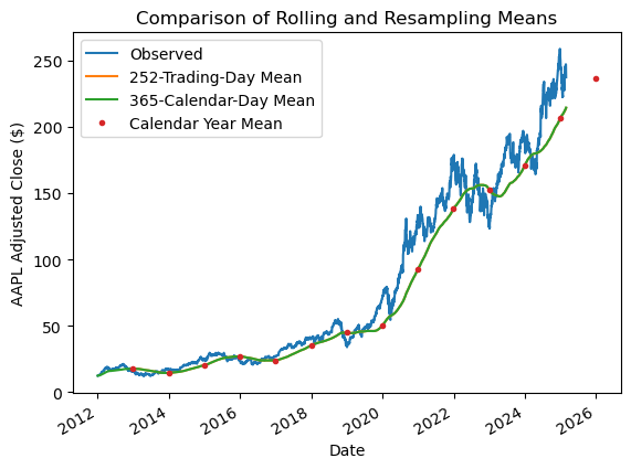
Note
If we specify the rolling window width as an integer:
- Each rolling window is that many observations wide and ignores time stamps
- Each rolling window must have that many non-missing observations
We can specify min_periods to allow incomplete windows. For integer window widths, min_periods defaults to the given integer window width. For string date offsets, min_periods defaults to 1.
Binary Moving Window Functions
Binary moving window functions accept two inputs. The most common example is the rolling correlation between two return series.
returns = df['Adj Close'].pct_change()returns| Ticker | AAPL | MSFT | SPY |
|---|---|---|---|
| Date | |||
| 1980-12-12 | NaN | NaN | NaN |
| 1980-12-15 | -0.0522 | NaN | NaN |
| 1980-12-16 | -0.0734 | NaN | NaN |
| 1980-12-17 | 0.0248 | NaN | NaN |
| 1980-12-18 | 0.0290 | NaN | NaN |
| ... | ... | ... | ... |
| 2025-02-21 | -0.0011 | -0.0190 | -0.0171 |
| 2025-02-24 | 0.0063 | -0.0103 | -0.0046 |
| 2025-02-25 | -0.0002 | -0.0151 | -0.0050 |
| 2025-02-26 | -0.0270 | 0.0046 | 0.0005 |
| 2025-02-27 | -0.0127 | -0.0180 | -0.0160 |
11143 rows × 3 columns
(
    returns['AAPL']
    .rolling(126, min_periods=100)
    .corr(returns['SPY'])
    .plot()
)
plt.ylabel('Correlation between AAPL and SPY')
plt.title('Rolling Correlation between AAPL and SPY\n (126-Day Window w/ 100-Day Minimum)')
plt.show()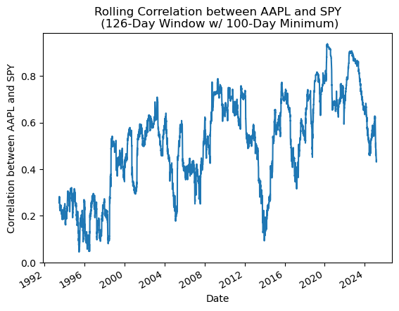
(
    returns[['AAPL', 'MSFT']]
    .rolling(126, min_periods=100)
    .corr(returns['SPY'])
    .plot()
)
plt.ylabel('Correlation with SPY')
plt.title('Rolling Correlation with SPY\n (126-Day Window w/ 100-Day Minimum)')
plt.show()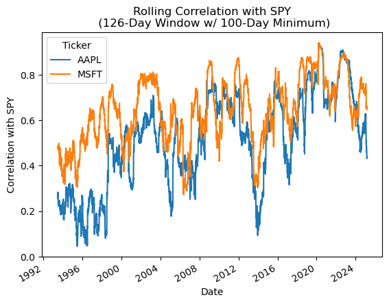
User-Defined Moving Window Functions
We can define our own moving window functions and use them with the .apply() method. However, note that .apply() method will be much slower than the optimized methods, like .mean() and .std(). Here, we will calculate rolling volatility with .apply() and .std() and compare their speeds.
(
    returns['AAPL']
    .rolling(252)
    .apply(np.std)
    .mul(np.sqrt(252) * 100)
    .plot()
)
plt.ylabel('Volatility (%)')
plt.title('Rolling Volatility\n (252-Day Window w/ 252-Day Minimum)')
plt.show()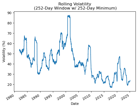
Do not be afraid to use .apply(), but realize that .apply() is often 1000 times slower than the optimized method!
%timeit returns['AAPL'].rolling(252).apply(np.std)2.28 s ± 109 ms per loop (mean ± std. dev. of 7 runs, 1 loop each)%timeit returns['AAPL'].rolling(252).std()613 μs ± 80 μs per loop (mean ± std. dev. of 7 runs, 1,000 loops each)References
McKinney, Wes. 2022. Python for Data Analysis. 3rd ed. https://wesmckinney.com/book/; O’Reilly Media, Inc.